Cover Sheet
Title
-
Identifying transcription start sites for Broad promoters using available combinations of evidence.
Objectives
-
Characterize a broad transcription start site (TSS) in a D. melanogaster ortholog
-
Use CAGE and RAMPAGE data to confirm the characterization of the D. melanogaster TSS
-
Use landmarks to set the boundaries of TSS search regions
-
Identify narrow and wide TSS search regions when blastn fails to localize the first transcribed exon
-
Use other lines of evidence to determine a wide TSS search region even when blastn succeeds in localizing the first transcribed exon
Prerequisites
Order
-
Overview of the challenges of annotating broad TSS
-
Define the search region for a broad promoter when blastn fails to localize the first transcribed exon (CG46466-RB)
-
Annotate a broad promoter when blastn succeeds in finding the first transcribed exon (myo-RA)
Class Instruction
-
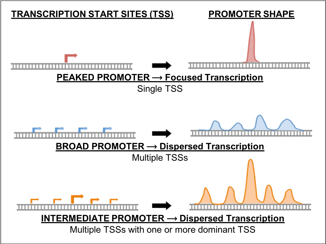
How are peaked and broad promoters different?
-
How do you use landmarks to set the boundaries of TSS search regions?
-
What is the relative ranking of pieces of evidence that can be used to identify narrow and wide TSS search regions of broad promoters?
-
Work through the Genome Browser examples for CG46466-RB in D. biarmipes.
-
Conclude by challenging students to identify the TSS search region for another D. biarmipes gene.
Applying various lines of evidence to rationally identify a TSS search region for genes with intermediate or broad promoters
In the previous modules in this series, we learned how to access information used to annotate a Transcription Start Site (TSS) for genes with a peaked promoter (Figure 1). However, genes with intermediate or broad promoters are often more difficult to annotate. These promoters have multiple TSSs and several lines of evidence must be used to define a search region for the TSS. This module will use several examples to illustrate strategies that you can use to define a search region and locate (annotate) the TSS or TSSs for these genes using the available evidence. In particular, F Element genes tend to have a higher probability of having broad promoters, making the challenge of annotating their TSSs more difficult. Moreover, on occasion you will run into a peaked promoter that is similarly troublesome to annotate and the strategies presented in this module can be applied to these genes.
Exercise 1: Classification of intermediate/broad promoters in D. melanogaster
-
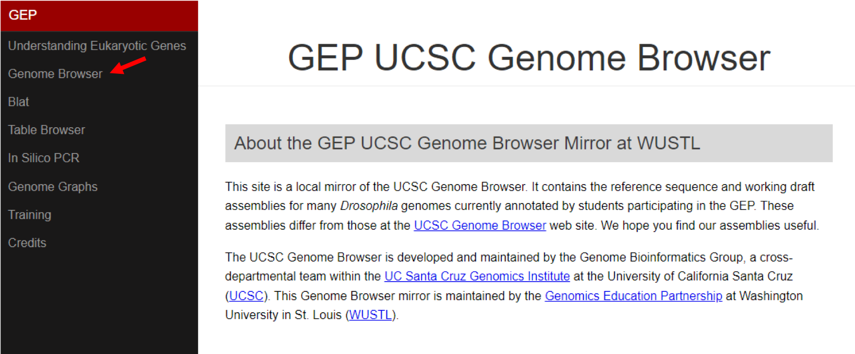
Let’s begin by classifying the promoter type of a D. melanogaster ortholog of the B isoform of the gene CG46466. Open a new web browser window and go to the Genomics Education Partnership (GEP) UCSC Genome Browser Mirror (Figure 2).
-
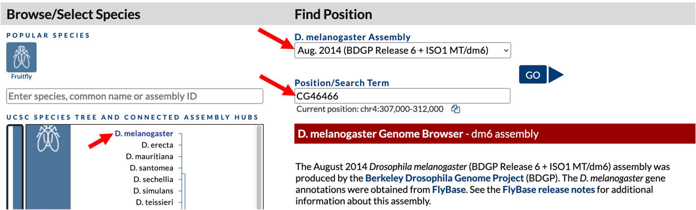
To navigate to the genomic region surrounding the CG46466-RB gene isoform in D. melanogaster, select “D. melanogaster” under “UCSC SPECIES TREE AND CONNECTED ASSEMBLY HUBS”, select “Aug. 2014 (BDGP Release 6 + ISO1 MT/dm6)” under the “D. melanogaster Assembly” field, and then enter “CG46466” under the “Position/Search Term” field. Click on the “GO” button (Figure 3).
-
The resulting page shows a list of the three CG46466 isoforms present in D. melanogaster. Click on the link for “CG46466-RB at chr4:661009-663124”. The CG46466 gene is located on chromosome 4 and the B isoform is located between nucleotides 661,009 and 663,124.
-
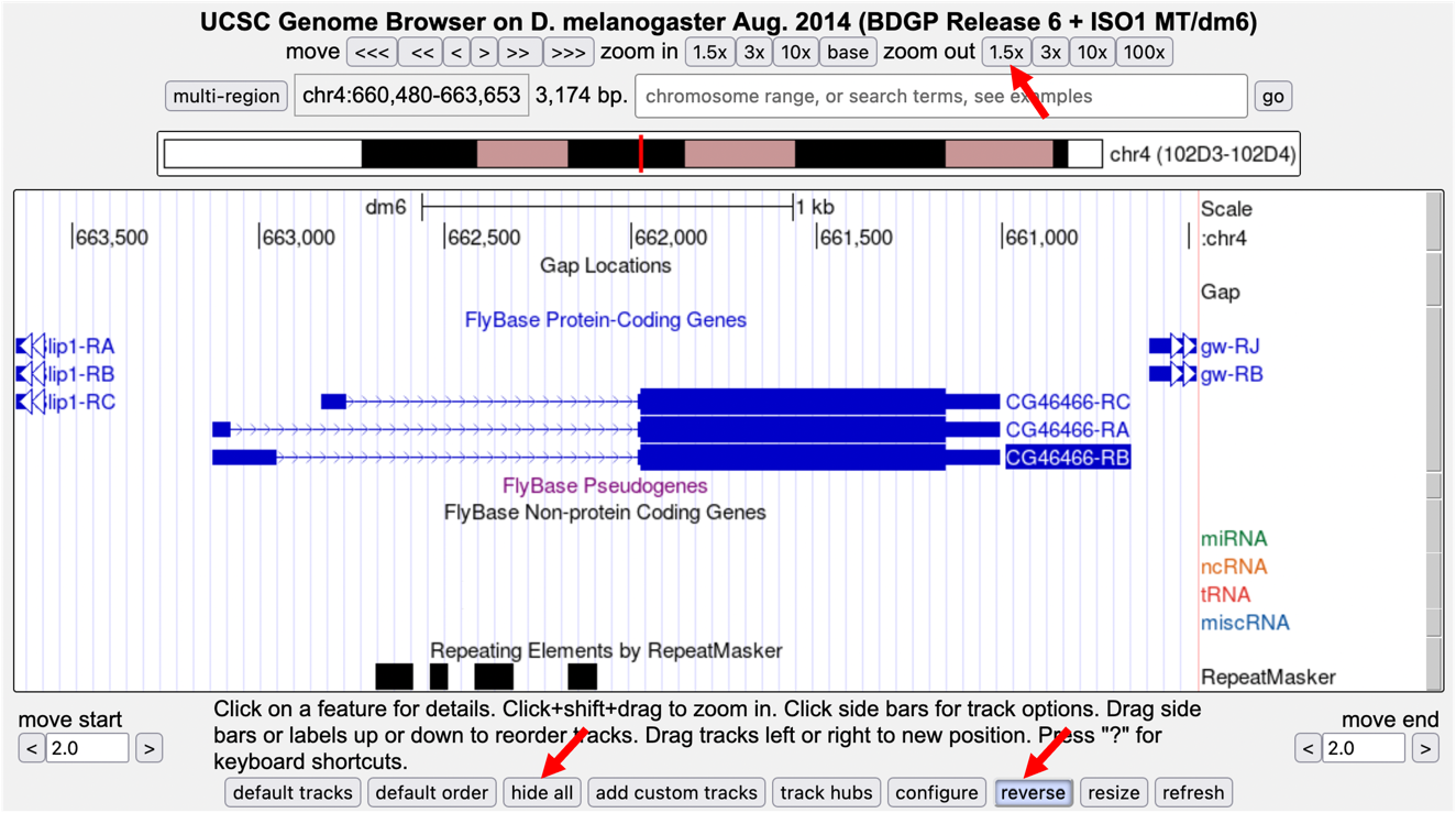
Zoom out 1.5X. The resulting genome browser window shows the genomic region that includes three isoforms of CG46466. The CG46466 gene is on the minus strand. To make it easier to interpret the evidence tracks, we will reverse complement the entire chromosome sequence. Click on the “reverse” button located in the display controls below the Genome Browser image (Figure 4).
-
Because the Genome Browser remembers the previous display settings, we will hide all the evidence tracks and then enable only the subset of tracks that we need. Click on the “hide all” button located below the Genome Browser image (Figure 4).
-
Next, we will display the evidence tracks that will allow us to characterize the type of promoter. Configure the display modes as follows:
-
Under “Mapping and Sequencing Tracks”
-
Base Position: full
-
-
Under “Chromatin Domains” Tracks
-
BG3 9-state (R5): dense
-
S2 9-state (R5): dense
-
-
Under “Gene and Gene Prediction Tracks”
-
FlyBase Genes: pack
-
-
Under “Expression and Regulation”
-
Detected DHS Positions (Cell Lines) (R5): pack
-
DHS Read Density (Cell Lines) (R5): full
-
TSS (Celniker) (R5): pack
-
-
-
Click any of the “refresh” buttons to update the display.
-
Since we want to characterize the promoter of the CG46466-RB isoform we will zoom in on that region surrounding exon 1 (a non-coding exon). Type “chr4:662,550-663,550” into the “chromosome range, or search terms, see examples” text box, and then click the “go” button (Figure 5).
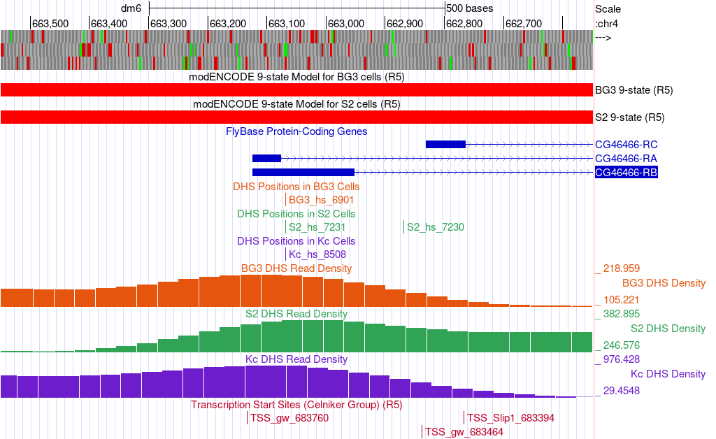
According the 9-state models for the CG46466-RB isoform, how is the chromatin state of this region classified?
|
|
Under “Chromatin Domains” click on the blue text for BG3 9-state or S2 9-state to see a chart that describes the different colors displayed in these tracks. |
How many DHS Positions (statistically significant DNase I hypersensitive sites) are located in this region?
How many TSSs were predicted in the Celniker data in this region?
D. melanogaster promoters are classified based on the number of annotated TSS (Celniker) positions and the number of DHS positions within a 300 bp window (Table 1). Type “chr4:662,969-663,268” into the “chromosome range, or search terms” text box, and then click on the “go” button. Based on the data, how should we classify the promoter of the D. melanogaster CG46466-RB gene?
| Promoter Shape | Criteria |
|---|---|
Peaked |
|
Intermediate |
|
Broad |
|
Insufficient Evidence |
|
-
In addition to the DHS sites and Celniker TSS predictions, we can also utilize CAGE and RAMPAGE data to support (or not, depending on the data) the characterization of the promoter. To view this data, we will add these tracks to the browser while keeping the tracks we loaded above. Configure the display modes as follows (Figure 6):
-
Under “Expression and Regulation”, click on the blue “Combined modENCODE CAGE TSS” link
-
Change the “Maximum display mode” to “full”
-
Scroll down to the “List subtracks” section and change the “modENCODE CAGE (Plus)” display mode to “hide” (or uncheck)
-
Scroll up to the top of the page, and then click on the “Submit” button.
-
-
Under “Expression and Regulation”, click on the blue “Combined RAMPAGE TSS (R5)” link
-
Change the “Maximum display mode” to “full”
-
Scroll down to the “List subtracks” section and change the “RAMPAGE (Plus)” display mode to “hide” (or uncheck)
-
Scroll up to the top of the page, and then click on the “Submit” button
-
-
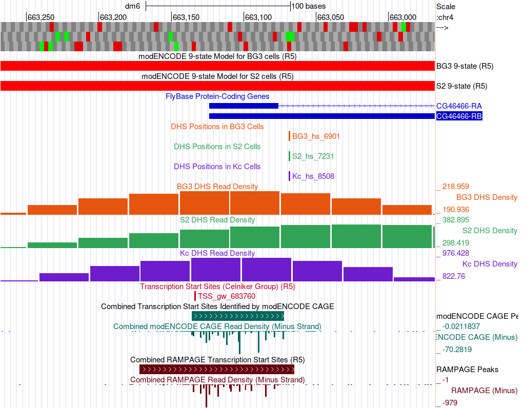
Why change the display of both the CAGE and RAMPAGE data to hide the data from the plus strand?
Do the CAGE and RAMPAGE data match with the locations of the Celniker predicted TSSs?
|
|
Use the browser to zoom in for a closer look if necessary. |
Are the CAGE and RAMPAGE data consistent with a peaked, intermediate, or broad promoter shape?
Which is the stronger evidence for the promoter shape — Celniker TSSs and DHS positions, or CAGE and RAMPAGE? Explain.
Ranking lines of evidence for determining the boundaries of TSS search regions
As part of the GEP TSS annotation projects, we marshal different lines of evidence to define the boundaries of the TSS search region for any given gene. Ideally, the data from these different sources should be in agreement. However, not all lines of evidence are equal.
The different lines of evidence that can be used to establish TSS search region boundaries are ranked below from most to least reliable:
-
blastn alignment of the 1st transcribed D. melanogaster exon
-
RNA Pol II X-ChIP-Seq
-
RNA-Seq (including splice junction predictions from TopHat and regtools)
-
Conservation
blastn alignment of the 1st transcribed D. melanogaster exon: The gold standard evidence for the location of the TSS for a GEP project gene is homology to the 1st transcribed exon of the ortholog in D. melanogaster. The blastn match should have a low E-value with a high sequence identity between the 1st transcribed exon in D. melanogaster and the GEP project sequence. In addition, the TSS shouldn’t need to be extrapolated by more than 150 bp from the end of the aligned sequence; and other lines of evidence (such as those described below) should agree with the proposed TSS position.
If blastn succeeds at finding the location of the first exon in the project sequence, then define the boundaries of the TSS search region as ±300 bp from the initial 5' nucleotide in exon 1. Typically, this will be the narrow search window annotation. Using the information contained in the tracks listed below may allow you to define a narrower search window, but most of the time if you find a blastn match, your annotation adventure can stop here!
Of course, blastn won’t always identify the location of the 1st transcribed D. melanogaster exon (when it fails one or more of the criteria listed above). Fortunately, other lines of evidence can be utilized to define a TSS search region.
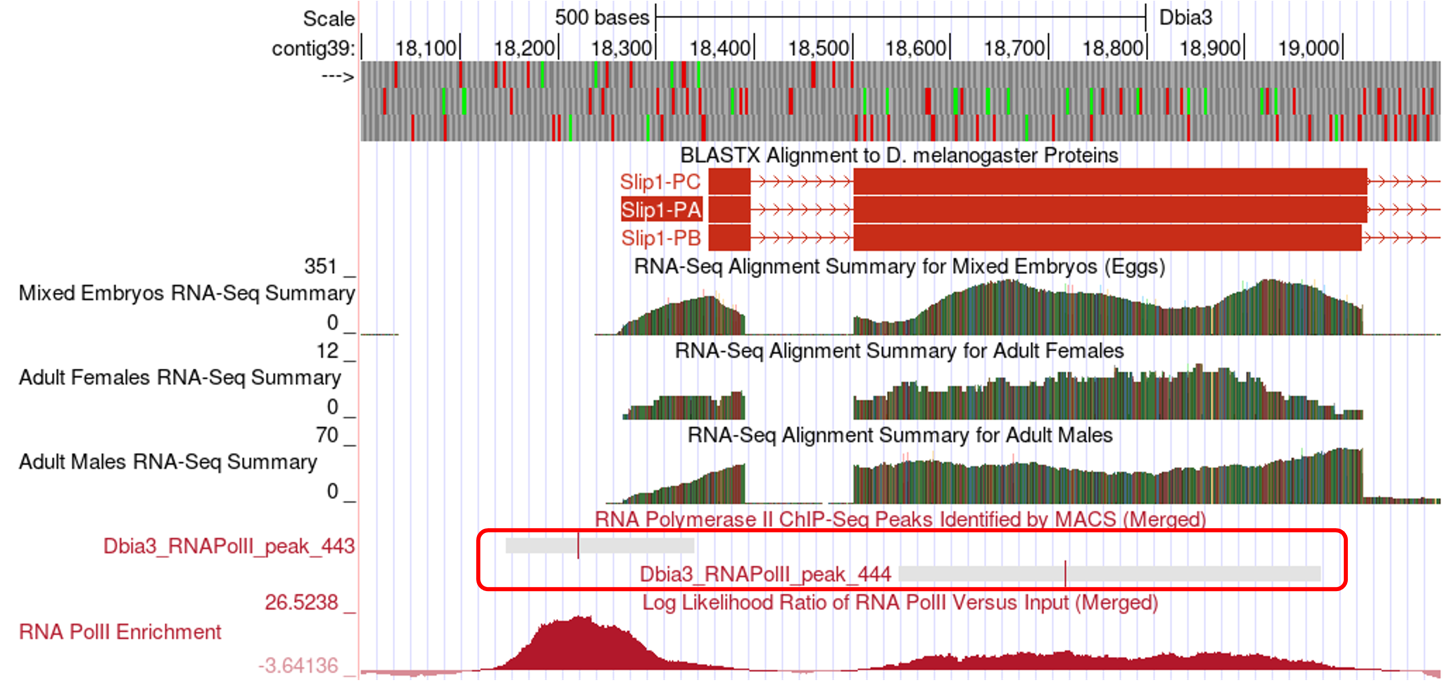
RNA Pol II X-ChIP-Seq: RNA Polymerase II (RNA Pol II) is the enzyme that transcribes protein-coding genes in eukaryotes and is often enriched near the TSS of a gene isoform. Researchers have used a technique called ChIP-Seq to identify regions in the genome where RNA Pol II is in fact enriched. Very briefly, chromatin (DNA and proteins) is fragmented to small size. RNA Pol II and the DNA that it is bound to is precipitated using an antibody specific to RNA Pol II. The DNA is then sequenced, and the reads are mapped back to the genomic sequence. Because the sequenced DNA corresponds to sites where RNA Pol II was bound, locations where RNA Pol II is enriched can be identified by a pile-up of reads called peaks (see the RNA Pol II Enrichment track).
The program that identifies peaks reports both the boundaries of the peak (grey bar), and a peak apex (vertical red line) where the pile-up is the highest (Figure 7). These peaks are a good proxy for the region that includes the TSS and can be used as very high-quality landmarks for defining a TSS search region. When defining a search region, the boundaries of the RNA Pol II peaks should be used rather than the peak apex.
RNA-Seq (including TopHat junctions): In RNA-Seq all of the messenger RNA is sequenced, and the reads are mapped back to the genome to identify the location of protein-coding genes. Furthermore, the program TopHat identifies reads that span exon junctions. These reads are displayed in the TopHat reads tracks.
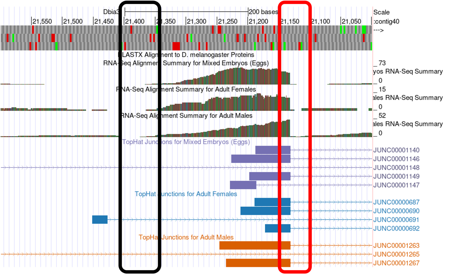
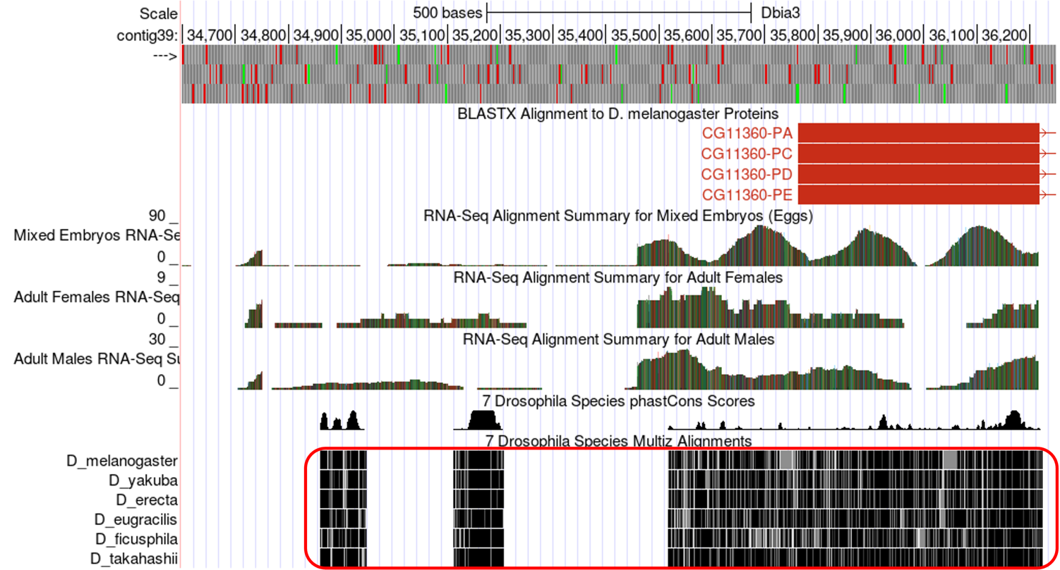
The RNA-Seq tracks can be very useful for determining a TSS search region. Often when blastn fails to identify the location of the 1st transcribed D. melanogaster exon, the RNA-Seq and TopHat tracks can be used to identify the approximate location of the first exon. Moreover, these tracks can be used to define a TSS search region. A tail of continuous RNA-Seq enrichment upstream of the initial (predicted) exon can be used to define the upstream boundary of a search region because this is indicative of where transcription for the gene began. In addition, TopHat junctions can be used to define the downstream boundary of a search region because, by definition the TSS must be upstream of the 3' splice site of the first exon. See examples of both of these types of regions in the boxed areas in Figure 8.
Conservation: Sequences in the genome that serve a function, like the sequence of a gene, tend to be conserved over evolutionary time. Therefore, we would expect that promoter and exon sequences would tend to be more highly conserved than surrounding sequences. The conservation tracks highlight conserved nucleotides between Drosophila species. If a nucleotide is conserved it is shaded black, so the more black nucleotides, the higher the degree of conservation (Figure 9). The boundaries of highly conserved regions can serve as landmarks for defining the boundaries of a TSS search region. However, this is the lowest quality evidence you can use for this task and should only be used if the other lines of evidence are completely lacking.
You can find more technical information about the evidence tracks described above by clicking on the text links for each track to read a brief summary of the track, and by reading the primary literature sources found on the track description page.
We use combinations of these evidence tracks to define the narrowest TSS search window possible (given the available evidence). A broad search window (600 bp or more) can also be defined by using landmarks in the different evidence tracks that are further apart from each other. In any event, both the narrow and broad search regions should be anchored to clear landmarks in the evidence tracks.
A quick note before we move on to some practice: In general, the alignments to D. melanogaster proteins and transcripts (i.e., the “D. mel Proteins” and “D. mel Transcripts” evidence tracks) make poor landmarks for annotation. The sequences of the untranslated regions of genes tend to diverge faster over evolutionary time than the coding regions of genes. For this reason, alignments are often only partial — particularly at the 5' end of the first transcribed exon where we expect to find the gene promoter. Hence, these alignments should not be used as annotation landmarks.
Exercise 2: Using evidence-based landmarks to define the boundaries of a TSS search region
As discussed above, when blastn fails to identify the location of the 1st transcribed D. melanogaster exon other lines of evidence must be used to define a TSS search region. When using these other lines of evidence, it is important to use clearly delineated landmarks in the evidence tracks to set the TSS search region boundaries in order to encourage consistency between different student annotators. In other words, we want to avoid defining the boundaries of a search region arbitrarily. In this exercise we will use an example to practice using landmarks found in the various data tracks to establish TSS search region boundaries that are well supported by experimental evidence.
The genomic region we will investigate is in the vicinity of the TSS of the myo gene on the D. biarmipes Aug. 2013 (GEP/Dot) contig40.
-
To navigate to this region, return to the Genome Browser Gateway page by following the directions above or by clicking on the “Genomes” link in the navigation bar at the top of the browser page. Change the species to “D. biarmipes” by clicking on the link in the tree on the left-hand side of the page. Change the “D. biarmipes Assembly” to “Aug. 2013 (GEP/Dot).” Type “contig40” into the “Position/Search Term” text box and click on the “GO” button to navigate to this contig.
-
Click “hide all” and configure the display modes as follows:
-
Click the “reverse” button in the tools below the browser window to display the reverse complement of the contig (if the browser is not already configured this way).
-
Under “Mapping and Sequencing Tracks”
-
Base Position: full
-
-
Under “Genes and Gene Prediction Tracks”
-
Reconciled Gene Models: pack
-
D. mel Transcripts: pack
-
-
Under “RNA Seq Tracks”
-
RNA-Seq Alignment Summary: show
-
RNA-Seq TopHat: pack
-
-
Under “Expression and Regulation”
-
RNA PolII Peaks: pack
-
RNA PolII Enrichment: full
-
-
Under “Comparative Genomics”
-
Conservation: pack
-
-
Click on any of the “refresh” buttons.
-
-
Finally, to zoom in to the region surrounding the TSS of the myo gene, type “contig40:20,400-22,100” into the “chromosome range, or search terms” text box and click the “go” button.
This should configure the browser to show an image similar to the one displayed in Figure 10. We have drawn lines to 10 potential landmarks in this image. Your task is to determine whether each of them are good landmarks for identifying a TSS search region based on the information presented in the section above. Feel free to use the browser tools to zoom in and out to look at each potential landmark (you can always return to this view by entering the coordinates listed above). Fill in the table for Question 9 with your observations.
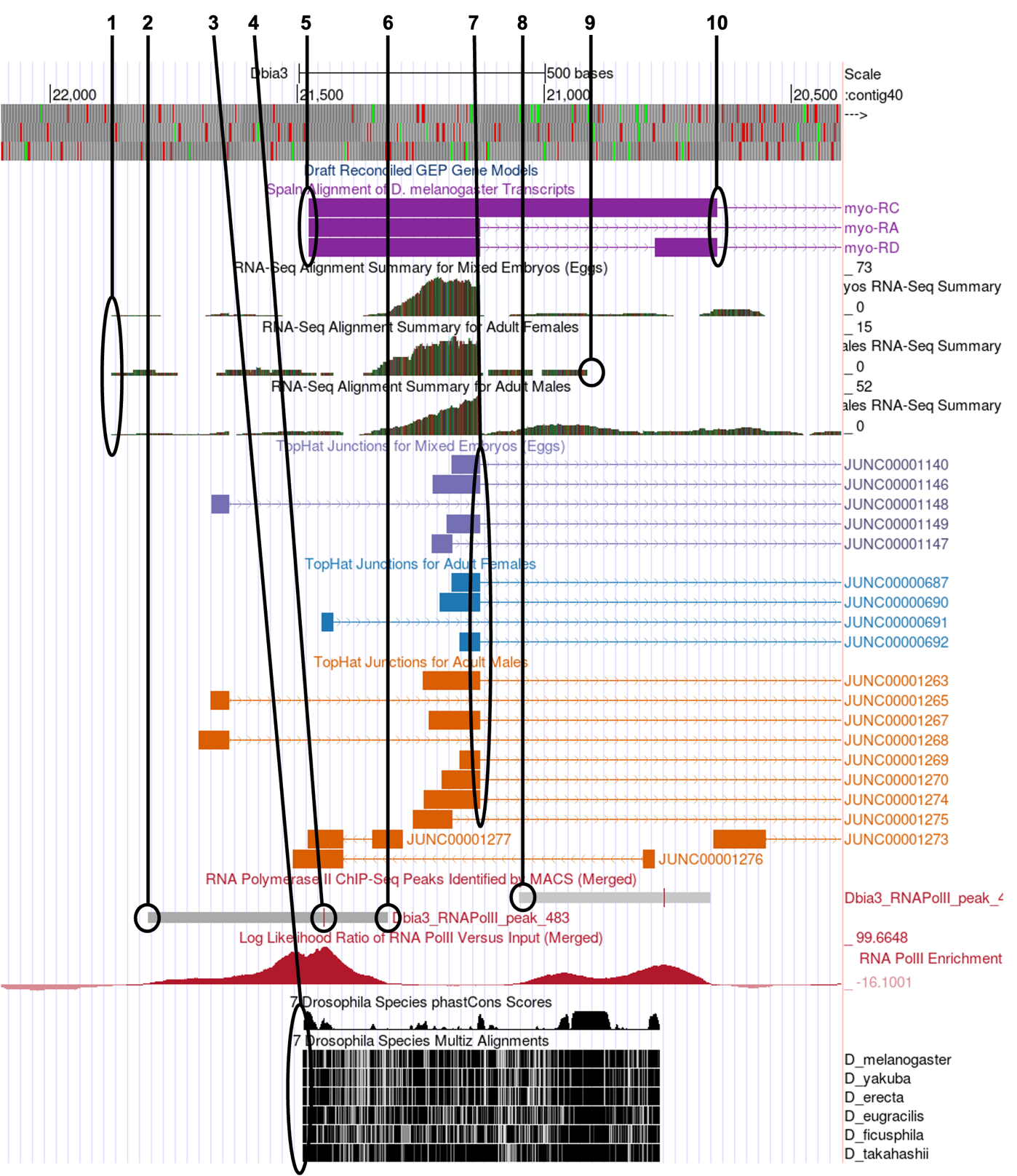
In Figure 10, numbered lines are drawn to ten potential landmarks in the vicinity of the TSS of the myo gene on contig40 (GEP/Dot) in D. biarmipes. Indicate the following for each in the table below: Is it a good landmark for TSS annotation? The quality of the landmark (use it 1st, 2nd or 3rd). Finally, provide a short explanation of your decision.
| # | Use as Landmark? Y/N | Use 1st, 2nd, 3rd | Explanation |
|---|---|---|---|
1 |
|||
2 |
|||
3 |
|||
4 |
|||
5 |
|||
6 |
|||
7 |
|||
8 |
|||
9 |
|||
10 |
Using the landmarks identified above, define the narrowest search region you can justify for the myo TSS or TSSs. Describe the landmarks you used to determine the search region.
|
|
Use the browser to zoom in and out to identify the precise boundaries to the nucleotide. |
Next, identify a wide search region for the myo TSS using the landmarks described above.
Homework: Determining a TSS search region for the D. biarmipes CG46466-RB gene
In exercise 1 we determined that the TSS of the B isoform of the CG46466 gene in D. melanogaster had a broad shape. Now that we have learned how to use evidence-based landmarks to set the boundaries of a TSS search region, let’s apply that knowledge to define a TSS search region for the CG46466-RB gene in the D. biarmipes GEP project sequence.
First, we will determine if we can locate the 1st transcribed D. melanogaster exon using BLAST.
-
Open a new browser tab and navigate to the NCBI BLAST home page. Click on the “Nucleotide BLAST” image under the “Web BLAST” section.
-
Check the box “Align two or more sequences”. An “Enter Subject Sequence” text box will appear.
-
Open a new browser tab and navigate to the Gene Record Finder on the GEP website. Enter “CG46466” into the search term box and click on “Find Record.”
-
Scroll down and click on the “Transcript Details” tab. By looking at the Exon Usage Map, we can see that the first transcribed exon of the B isoform of CG46466 is exon 1. Scroll down to the exon table and click on the first row (FlyBase ID = 2). A window will open that contains the sequence of exon 1.
-
Copy and paste the exon 1 sequence for D. melanogaster CG46466-RB into the “Enter Query Sequence” text box in BLAST.
-
The CG46466 gene is encoded on the F Element in D. biarmipes so to navigate to this sequence, simply type “contig38” into the “chromosome range, or search terms” text box in the GEP UCSC Genome Browser and click on the “go” button.
-
Alternatively, if you do not have the GEP UCSC Genome Browser still open from the previous exercise, direct your browser to the GEP UCSC Browser Gateway page as described above. Click on “D. biarmipes” in the list of organisms, select “Aug. 2013 (GEP/Dot)” under the “D. biarmipes Assembly” then type “contig38” into the “Position/Search Term” field and click on the “GO” button.
-
-
Retrieve the DNA sequence of this contig by clicking on “View” in the navigation bar at the top of the GEP UCSC Genome Browser page and then clicking on “DNA”. Copy the entire sequence and paste it into the “Enter Subject Sequence” text box in BLAST.
-
Reconfigure the BLAST settings as follows:
-
Program Selection: Somewhat similar sequences (blastn)
-
Under Algorithm parameters:
-
Expect threshold = 10
-
Word size = 7
-
Match/Mismatch Scores = 1,-1; Gap Costs = Existence:2 Extension:1
-
Filter = Uncheck Low complexity regions
-
-
-
Check “Show results in a new window” and click on “BLAST.”
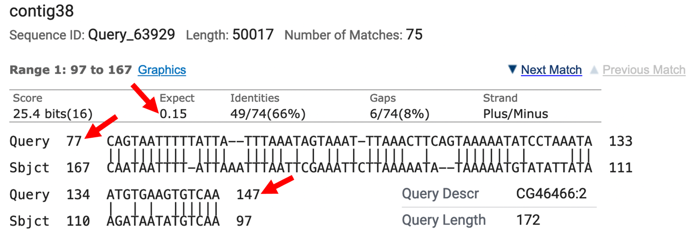
Was blastn able to locate the CG46466-RB exon 1 in the D. biarmipes contig38 project sequence? Explain the evidence you used to make this determination.
SPOILER ALERT
So (as you might have guessed, because otherwise why would we be doing this particular gene!), because blastn fails to localize the 1st transcribed D. melanogaster exon for the B isoform of the CG46466 gene in the D. biarmipes contig38 project sequence (Figure 11) we will have to use other pieces of evidence to determine a TSS search region for this gene.
-
If necessary, reconfigure the display of contig38 as follows:
-
Click the “reverse” button in the tools below the browser window to display the reverse complement of the contig (if the browser is not already configured this way).
-
Under “Mapping and Sequencing Tracks”
-
Base Position: full
-
-
Under “Genes and Gene Prediction Tracks”
-
D. mel proteins: pack
-
D. mel Transcripts: pack
-
-
Under “RNA Seq Tracks”
-
RNA-Seq Alignment Summary: show
-
RNA-Seq TopHat: pack
-
-
Under “Expression and Regulation”
-
RNA PolII Peaks: pack
-
RNA PolII Enrichment: full
-
-
Under “Comparative Genomics”
-
Conservation: pack
-
-
-
Click on any of the “refresh” buttons.
-
Now let’s investigate the 5' end of the CG46466 gene cluster. First, let’s take a broad overview of the region in order to get ourselves oriented. Enter “contig38:26,000-32,500” into the “chromosome range, or search terms” text box and click on the “go” button.
Now we can see displayed the beginnings of the coding DNA sequence (CDS) of the CG46466 isoforms (red tracks at the top) along with the Spaln alignment of D. melanogaster transcripts (purple tracks) (Figure 12). Spaln is a program that aligns the RNA sequences of many genes from a species (in this case D. melanogaster) against the genome of another (in this case the GEP D. biarmipes project sequences). The Spaln alignments can help us zero in on a region that may contain the TSS for a gene, but as mentioned above should not be used to set the boundaries of a search region.
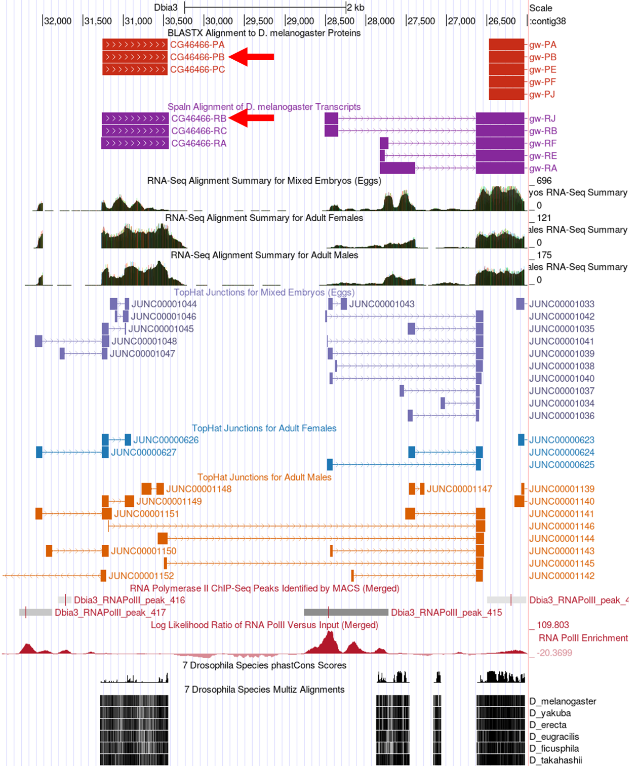
At which coordinate does the coding DNA sequence (CDS) of all of the CG46466-RB isoform begin (ATG codon)?
According to the Spaln alignment CG46466-RB seems to have only a single exon. What are the coordinates of this exon?
-
Using the Spaln alignment to guide us, let’s zoom in to that region further upstream. Enter “contig38:30,000-32,500” into the “chromosome range, or search terms” text box and click on the “go” button.
Now we can clearly see the region surrounding the CG46466-RB exon (Figure 13).
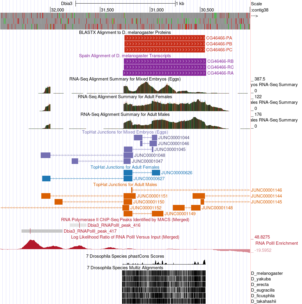
Can you conclude that the 5' end of the first CG46466 exon is located near the Spaln alignment or is other evidence present that would lead you to conclude that the first exon is actually in a different position? Explain.
-
Next, zoom into the upstream region by entering “contig38:31,850-32,400” into the “chromosome range, or search terms” text box and click on the “go” button (Figure 14).
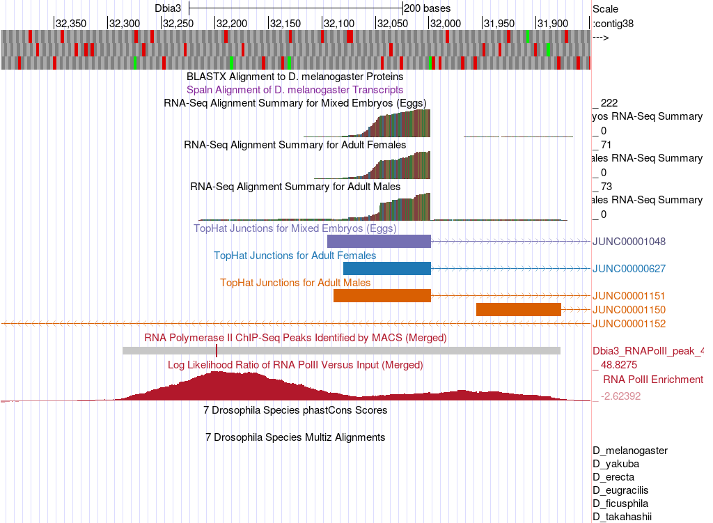
Based on the data available in this region, designate a narrow TSS search region for the D. biarmipes CG46466-RB isoform. Describe the landmarks you used to determine these search regions.
|
|
Use the browser to zoom in and out to identify the precise boundaries to the nucleotide. |
For the CG46466-RB isoform would it make sense to use the entire RNA Pol II peak to designate a wide TSS search region? Explain why or why not.
Finally, a nice feature of the D. biarmipes projects is that all of the consensus promoter motifs have been identified and assembled into an individual track that can be displayed in the browser. Therefore, we can visualize all of these motifs in a single step, without needing to search for each of them individually using Short Match (Figure 15). There are individual tracks for the motifs found on either the plus or minus strand. Since the CG46466 gene is encoded on the minus strand of contig38 we will only display the motifs on that strand. Bring up this track by configuring the browser display modes as follows:
-
Under “Mapping and Sequence Tracks”
-
Core Promoter Motifs (Minus): pack
-
-
Click on “refresh”
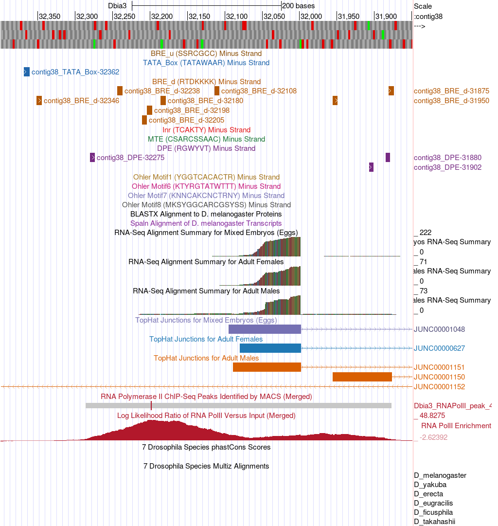
List all of the consensus promoter motifs found in the narrow TSS search region you identified in the previous question (include the start position of each motif).
Conclusion
In this module we have learned how to utilize different lines of evidence to annotate a TSS search region for broad promoter type genes, particularly when blastn fails to locate the 1st transcribed D. melanogaster exon in your project sequence. The strategy presented here relies on making use of the RNA Pol II X-ChIP-Seq data, RNA-Seq and TopHat data and Conservation to rationally assign the boundaries of a TSS search region using evidence-based landmarks in these data types. This strategy should be applicable to a wide range of GEP project TSS annotation problems.
If you would like further practice annotating this type of TSS, try doing CG33941 in either the D. biarmipes or D. elegans projects.