Prerequisites
Resources & Tools
-
All links for this lesson can be found on the Parasitoid Wasps Project page of the GEP website.
Introduction
This exercise will walkthrough an example of annotating a wasp venom gene. What does it mean to annotate a gene? When you look at a gene in the Genome Browser, you can look at the evidence tracks to identify the start and stop codons, the introns, exons, and UTRs. Annotation is the process of identifying those features in a gene. Using many types of data and your understanding of genetics, you will determine the most likely structure of an unstudied gene.
If you haven’t done gene annotation before, you might be surprised to learn that we don’t automatically know this kind of information about every gene. The parasitoid wasp genomes used in this project are draft genomes; these genomes still have significant errors. Furthermore, most of the analysis of the genes in these genomes has been done by computer algorithms. You will be one of the first people to ever pay serious attention to the gene you annotate. Those algorithms do a good job of finding gene sequences, but it takes human analysis to complete the annotation to high quality.
This walkthrough will discuss wasp versions of common Genomics Education Partnership (GEP) annotation tools—Genome Browser, Gene Record Finder, and Gene Model Checker—and provide background for the interpretation of data tracks that are unique to the Parasitoid Wasps Project.
|
|
The figures have been configured to fit this document while still maintaining readability; therefore, your screen may differ slightly. Commas have been included with all coordinates to improve readability, but you do not have to enter them in the Genome Browser (i.e., navigation will work the same with or without commas). |
Evidence for Gene Models
-
Conservation
-
Sequence similarity to genes in Nasonia vitripennis and/or Drosophila melanogaster
-
-
Expression data
-
RNA-Seq, EST, cDNA
-
-
Computational predictions
-
Open Reading Frames (ORFs); gene and splice site predictions
-
Basic Annotation Workflow
The following annotation workflow is optimized for genes encoding proteins with homology to the reference organism Nasonia vitripennis. Please consult with your instructor if your gene does not fit this category.
-
Identify the likely N. vitripennis ortholog
-
Observe the gene structure of the ortholog
-
Map each exon to the project sequence
-
Determine the exact coordinates of each exon
-
Verify the model using the Gene Model Checker
Accessing the Wasp Genome Browsers
Navigate to the wasp Genome Browsers, available through the UCSC Assembly Hubs for Parasitoid Wasps link. You can select any of the wasp genomes from the drop-down menu and paste a gene ID into the position box to be taken to the relevant genome region. Please note that N. vitripennis is the closest reference genome for this project.
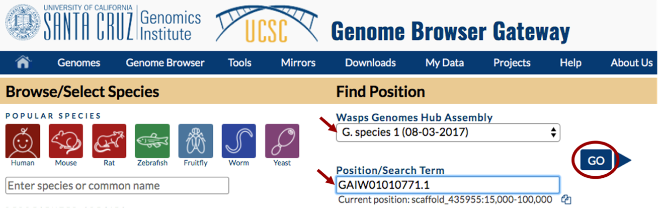
For this walkthrough, choose “G. species 1 (08-03-2017)” under the “Wasp Genomes Hub Assembly” drop-down menu and enter “GAIW01010771.1” in the “Position/Search Term” box (Figure 1). This is the 2017 assembly of the Ganaspis sp. G1 genome.
Configure the Browser
Set up your browser as follows:
-
Hide all
-
Mapping and Sequencing tracks: set Base Position: full
-
Transcript and Protein alignments tracks: set G1 Transcriptome: pack, D. mel FlyBase Proteins and N. vit Proteins (SPALN): pack
-
Gene Predictions (Species-specific Parameters) tracks: set Augustus Genes (BUSCO), N-SCAN Genes: pack
-
RNA-Seq tracks: set Unpaired Coverage and Paired-end Coverage: full; set Splice Junctions and StringTie Transcripts tracks: pack
-
Mass Spectrometry: set G1 Venom Proteins: pack
-
Click on any of the Refresh buttons
The Genome Browser will be centered on the GAIW01010771.1 gene model (Figure 2).
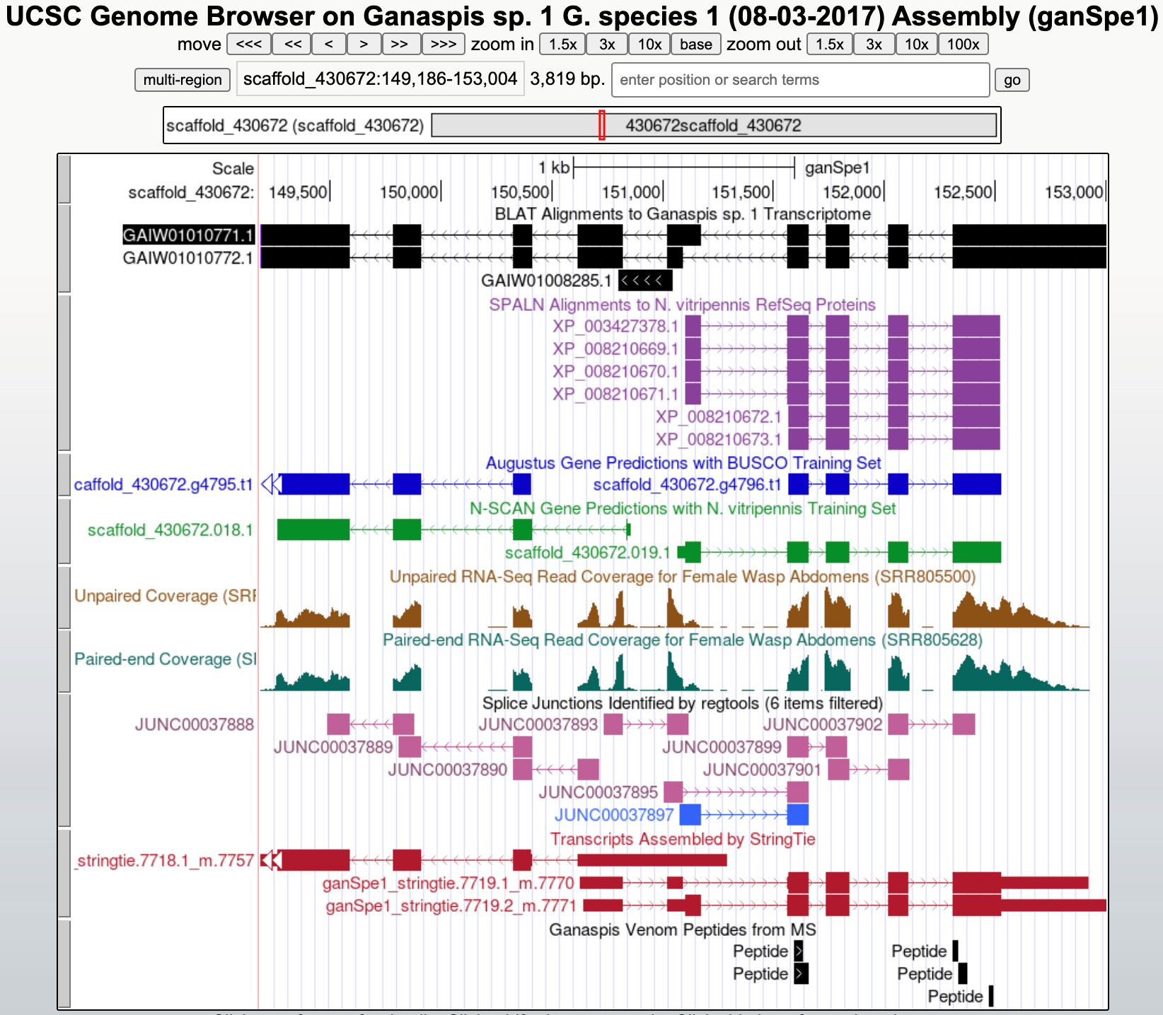
Interpreting the Transcriptome Track
A transcriptome is a list of all the mRNA sequences from a sample. That is information that can be very useful in identifying exon sequences. However, transcriptome data sets are never perfectly complete or free of errors, so they can’t be taken as absolute truth. To make the transcriptome data useful for annotation, the mRNA sequences have been compared to the genomic DNA sequence with a tool called BLAT. BLAT finds regions of highly similar sequences. Often that will indicate that a particular mRNA was transcribed from that genomic DNA.
Each wasp species will have a track that shows the BLAT alignment of a de novo assembled transcriptome with the genome sequence and is named <Species> Transcriptome — in the example above it is “G1 Transcriptome”. These de novo assemblies were previously used to identify wasp venom proteins. These transcripts are used as the starting point for the gene annotation, but please note the following:
-
These transcripts are often incomplete.
-
The RNA-Seq data was unstranded. This means that the “direction arrows” given in the track are NOT accurate; therefore, you should not use this track to determine whether the gene is on the plus or minus strand of the genomic DNA. Use the other data (i.e., StringTie, gene predictors) instead.
-
To find regions of similarity, BLAT needs a decent amount of sequence to compare. Short sequences, like exons that are smaller than 20 nucleotides, can be especially difficult for BLAT to find.
Interpreting the Mass Spectrometry Track
Another data track unique to the wasp project is the Mass Spectrometry track. Mass spectrometry gives the amino acid sequence of short fragments of a protein. In this case, the proteins were purified from the wasps' venom. Using a comparison tool similar to BLAT, these protein sequences have been matched to the regions of the genome that could have coded for them. These data will likely be very helpful in defining wasp venom genes, in particular de novo or highly diverged genes. For genes with multiple isoforms, you will also be able to assess whether the peptide data supports the hypothesis of a venom-specific isoform. For full details about the transcriptome and mass spectrometry, please see [Mortimer et al., 2013] and [Goecks et al., 2013].
Annotation: Identification of the Putative Homolog
Take a look at the different tracks displayed on the viewer window. Information on data provided by the different tracks can be found by hovering over the left-hand sidebar name of the track and then clicking on the grey pop-up text, or by clicking on the header for the drop-down control for that track (refer to UEG Module 1).
The most relevant tracks for your annotation are:
-
The SPALN alignments show protein sequences from both the reference genome (N. vitripennis) and D. melanogaster, aligned against your genome project assembly.
-
The gene predictor tracks, which attempt to identify areas in your project that may contain genes based on the N. vitripennis training set.
-
The tracks under the RNA-Seq section:
-
RNA-Seq tracks (unpaired and paired-end coverage), which indicates the location and abundance of RNA reads mapped against the project genome.
-
Splice junctions, which shows the exon junctions extracted from spliced RNA-Seq reads that have been aligned to the genome.
-
StringTie transcripts, which shows the RNA-Seq transcripts assembled by StringTie algorithm.
-
-
The G1 venom peptides show the mass spectrometry results for venom peptides, (i.e., proteins found in purified venom).
The goal at this stage is to determine if your project contains genes with homology to the reference genome, N. vitripennis and/or D. melanogaster (orthologs) to aid in your annotation using comparative genomics. One good place to start is by looking for hits in the SPALN tracks, either from N. vitripennis reference genome or from the annotated proteins of D. melanogaster. These hits indicate that the DNA in the matched regions encodes a protein with similarity to those in N. vitripennis and/or D. melanogaster, and therefore could be an ortholog.
In this example, only alignments to proteins in the RefSeq database of N. vitripennis are found under the SPALN tracks. There are no alignments against D. melanogaster proteins in FlyBase. Click on the protein ID (circled in Figure 3) to the left of the longest alignment.
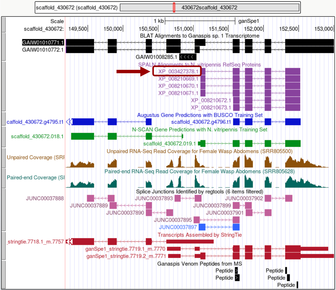
In the “Item Details” page, click on the “XP_003427378.1” link under the “NCBI Details” field to view the NCBI protein record for the isoform you selected (Figure 4).

|
|
Some of the reference sequences for Nasonia have been removed from the NCBI database. Students can refer to the archived, “obsolete version” to find the locus ID to use for Gene Record Finder (Figure 5). |
Scroll down to “CDS” feature to find the gene name associated with that protein isoform: “LOC100677983” (Figure 6).
If your project does not show any hits under the SPALN tracks, you can activate the TBLASTN tracks under the “Transcript and Protein Alignments” section or perform a tblastn search of N. vitripennis proteins database using one of the gene predictors features as a query; choose preferably a prediction that best aligns with venom peptides, the G1 Transcriptome, and the StringTie predictions. Please consult with your instructor on how to perform that search.
Determine the Gene Structure
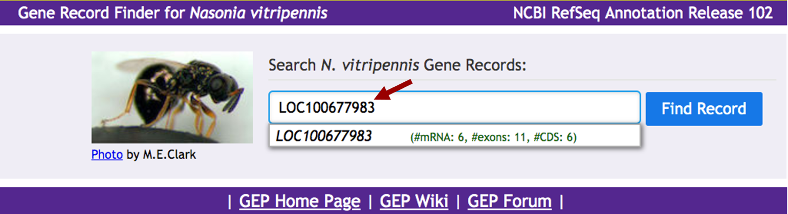
Open a new web browser tab and navigate to the Gene Record Finder for Nasonia vitripennis and paste the gene name in the search box and then click on the “Find Record” button (Figure 7).
This tool is used for determining the number of isoforms in the parasitoid wasp reference genome (Nasonia vitripennis). Knowing the number of isoforms in the reference wasp species will help guide the annotation process in G1 species, since we assume a certain level of evolutionary conservation.
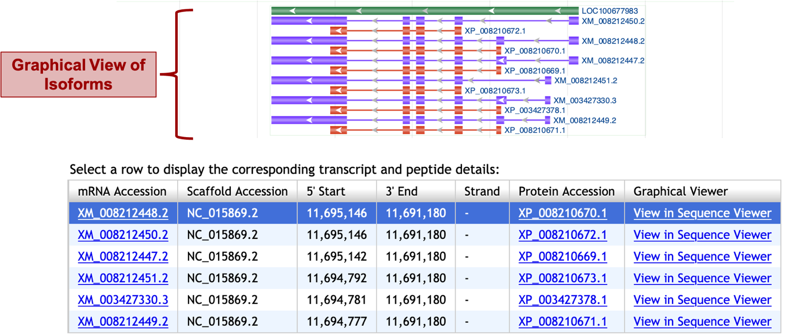
Gene Record Finder shows that the N. vitripennis LOC100677983 has six isoforms. Figure 8 below shows a graphical view of the isoforms (top) and a list form (bottom). The purple features (XM_ prefix) show the transcript isoforms which are all different and the red features show the corresponding polypeptides (XP_ prefix). Exons are depicted by boxes that are connected by introns shown as lines.
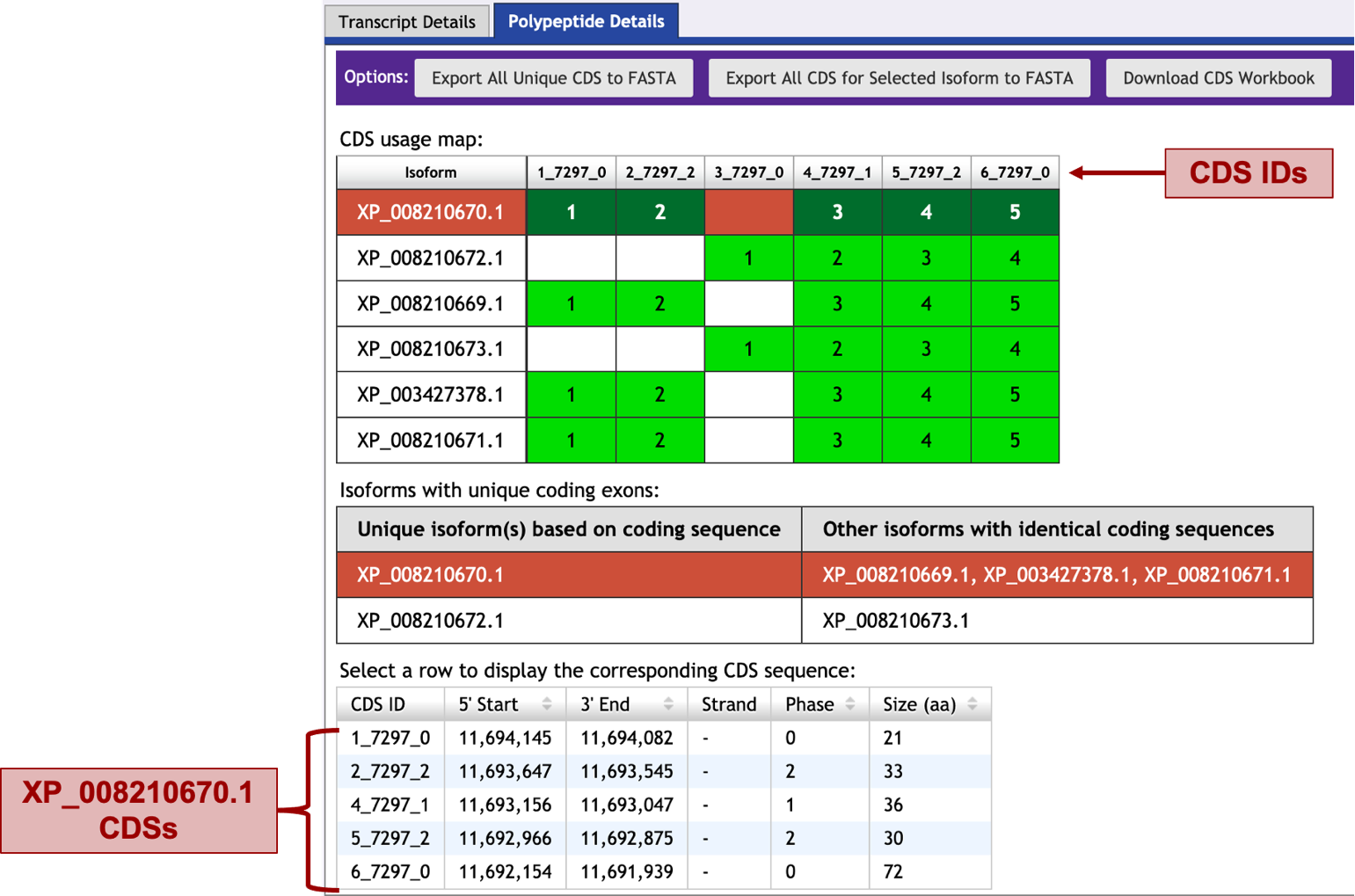
Annotation of All Non-identical Isoforms
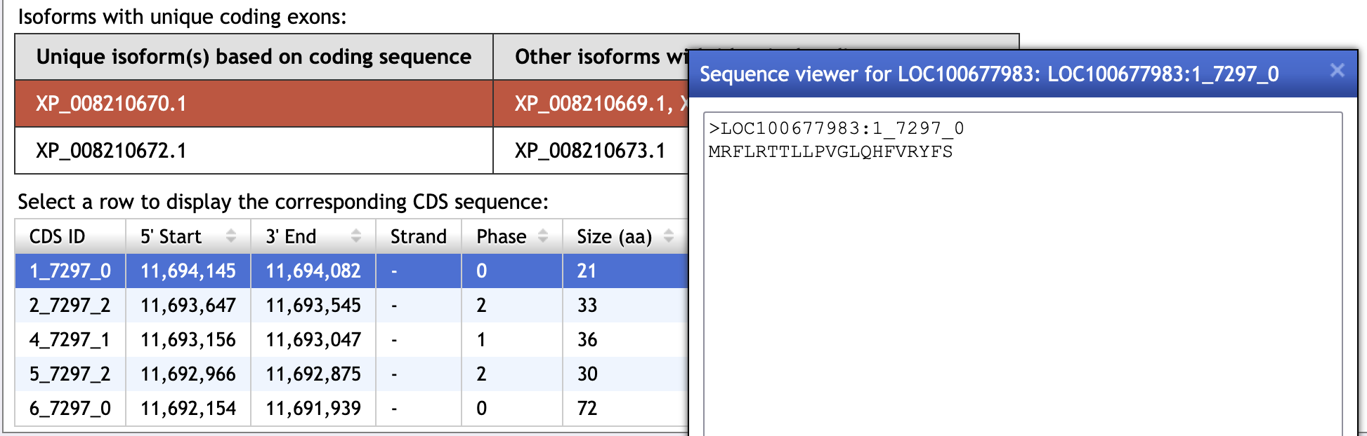
To start this process, in the Gene Record Finder window scroll down to the bottom of the page. The last section there has two tabs: “Transcript Details” and “Polypeptide Details” (Figure 9). Make sure the “Polypeptide Details” tab is selected (Isoforms will have “XP_” prefix). The “CDS usage maps” table shows the list of all the isoforms and their coding exons (CDSs) as green blocks. Each coding exon is labeled at the top of the table with its ID number. Some of the coding exons, for example 4_7297_1, are present in all the isoforms; others, for example 3_7297_0, are only present in some of the isoforms (Figure 9). Isoform XP_008210670.1 has five coding exons, and isoforms XP_008210669.1, XP_003427378.1, and XP_008210671.1 all have those same coding exons. Similarly, isoform XP_008210672.1 and isoform XP_008210673.1 both share the same four coding exons. Thus, you will annotate the two non-identical isoforms XP_008210670.1 and XP_008210672.1; annotate the longer isoform first (XP_008210670.1). Under the CDS usage map section, clicking on the XP_008210670.1 isoform, will display the information of the five coding exons on a table at the bottom of the screen: their IDs, the start and end coordinates in the chromosome of the reference species (N. vitripennis), the strand from which they are transcribed, and their size.
Exon by Exon Mapping to the Project DNA
You will now start mapping each coding exon for XP_008210670.1 (one of the two unique isoforms of N. vitripennis) to your Ganaspis sp.1 project to identify the approximate coordinates where they match. Because you will be running several BLAST searches against the same project sequence, it will be convenient to have this sequence saved in a file.
-
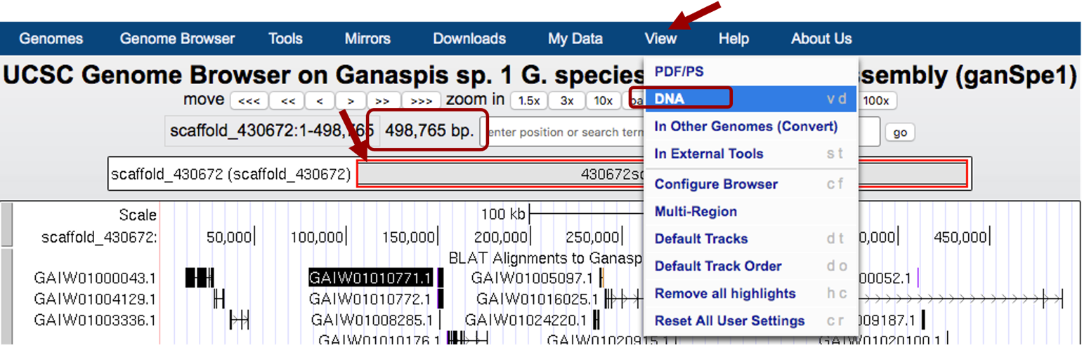
Create a .txt or .fasta file with the DNA sequence of the scaffold from G. species: Go to the Genome Browser and zoom out 100% (you need to click 2 or 3 times) until you see the box with the red outline covering the entire length of the project (Figure 10). You will also know you have the entire project when the number of base pairs is 498,765.
Then from the menu bar at the top of the screen click on “View” and choose “DNA Sequence” from the drop-down menu options (Figure 10). In the new window that opens, under “Sequence Formatting Options”, select “Get DNA”, which will display the DNA sequence for the entire project (scaffold_430672) — copy and paste the scaffold sequence in a text editor (Notepad, TextEdit) or Word document and save it as a txt file (scaffold_430672_ganSpe1.txt) or fasta file (scaffold_430672_ganSpe1.fasta) on your computer.
-
Obtain the protein sequence of the 1st exon from N. vitripennis to perform the search against the G. species scaffold. To obtain the protein sequence of the first CDS for this isoform, go back to the Gene Record Finder page, scroll down to the table at the bottom of the screen and select the first row. A pop-up window will show the corresponding CDS sequence (Figure 11). Copy the sequence.
-
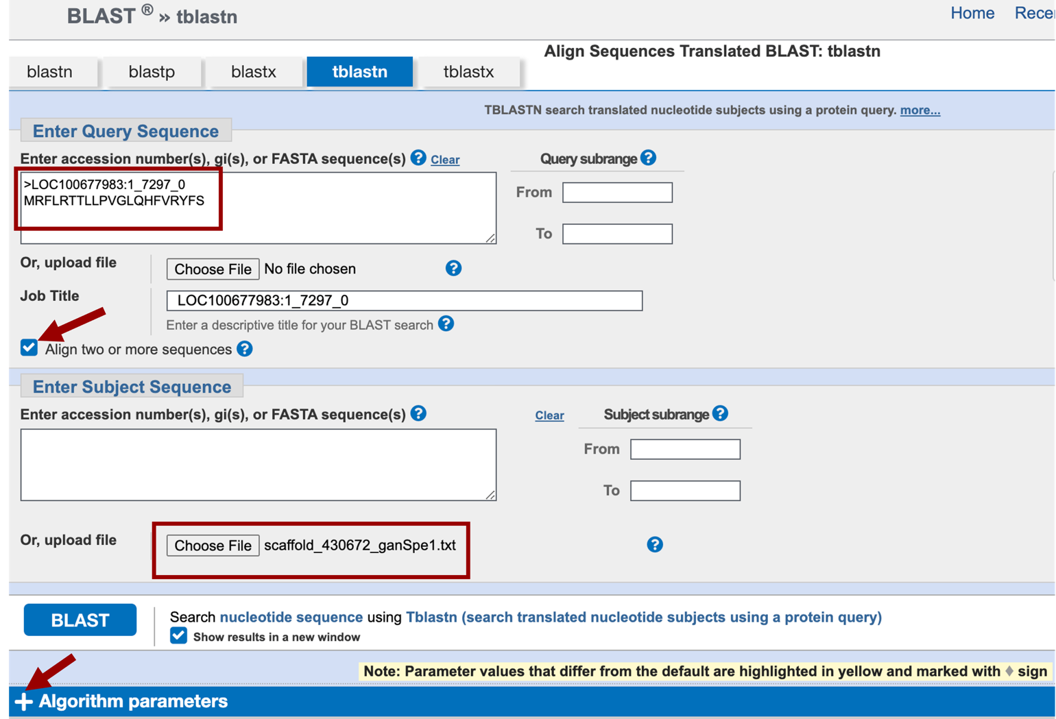
tblastn BLAST search: Open a new web browser tab and navigate to NCBI BLAST. Click on “tblastn”, which will allow us to compare a protein sequence (the CDSs) to a translated nucleotide sequence (our project). On the resulting page, paste the copied CDS sequence into the top box under the “Enter Query Sequence” section, and click on the box labeled “Align two or more sequences”. Under the “Enter Subject Sequence” section, click on the “Choose File” or the “Browse” button, and select the scaffold_430672_ganSpe1 sequence file on your computer.

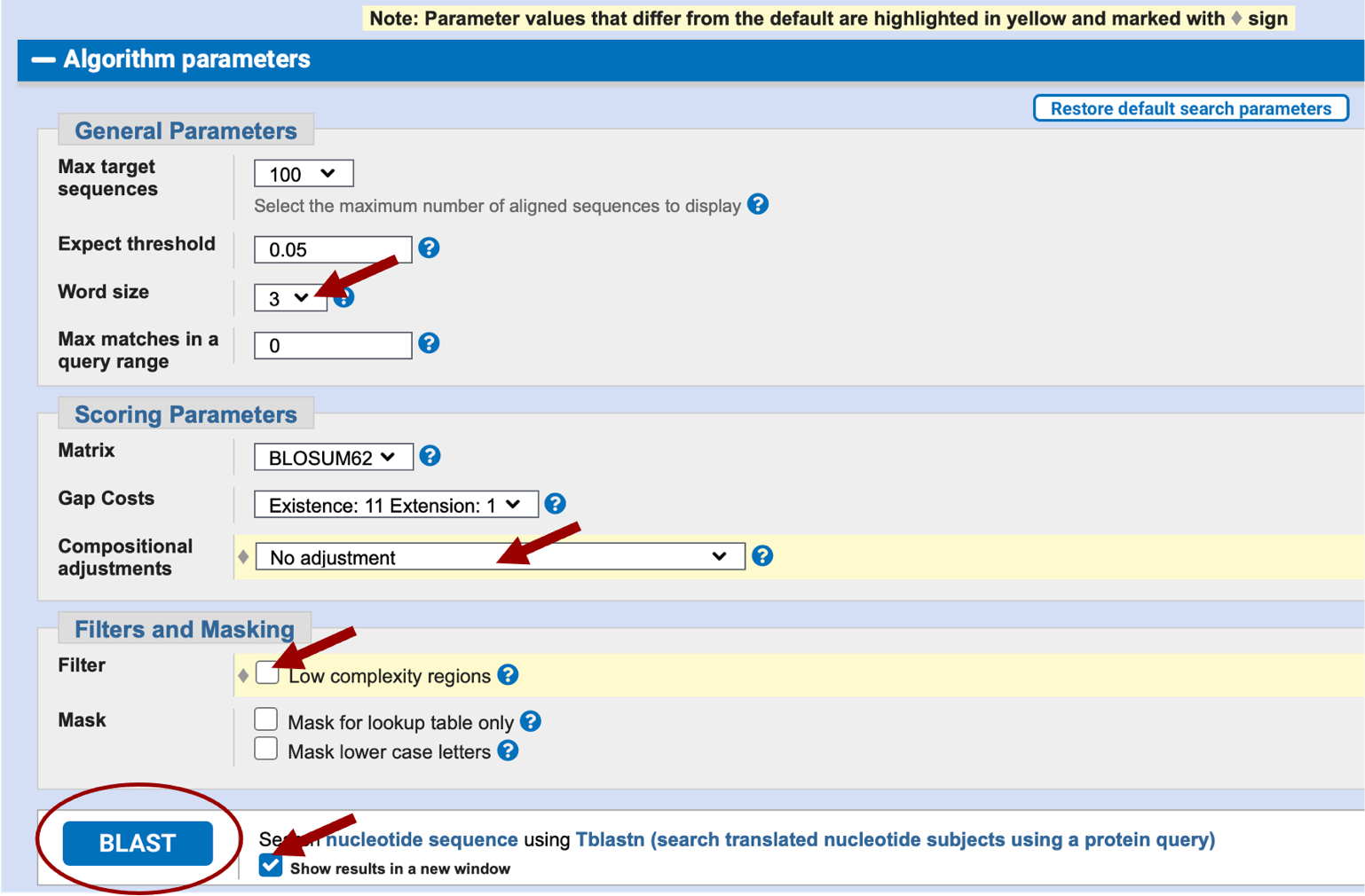
You could have used blastx search, but in that case, you would have used your scaffold sequence as the query sequence and the CDS as the subject sequence. Click on the “Algorithm parameters” link below the BLAST button to expand this section (Figure 12). Change the “Compositional adjustments” field to “No adjustment” and uncheck the “Low complexity regions” filter under the “Filters and Masking” section. Verify the word size is 3. For convenience, check the “Show results in a new window” box next to the BLAST button and you will be able to reuse this window to run BLAST for the remaining exons. Click on “BLAST” (Figure 13).
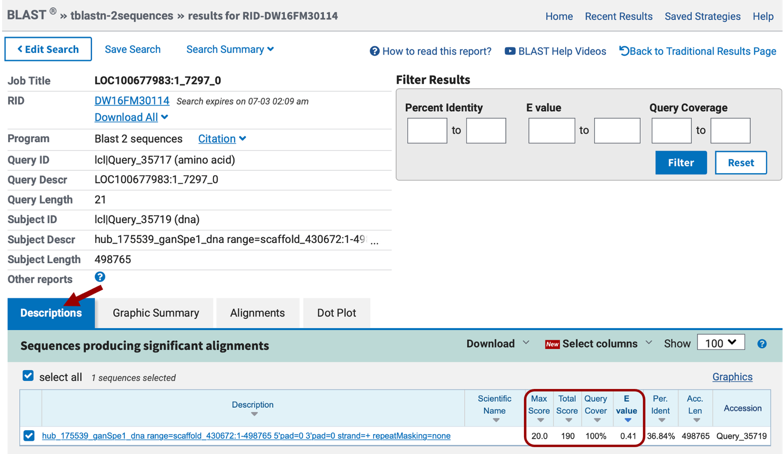
The BLAST results page will return a “No significant similarity found” message meaning, under these parameters, nothing in the translated scaffold_430672 sequence of Ganaspis sp. 1 had similarity to the first exon of XP_008210670.1 from N. vitripennis.
Change the “Expect threshold” field value to 10 and then repeat the tblastn search. Lower Expect thresholds are more stringent, leading to fewer chance matches being reported, increasing the Expect threshold will increase the number of matches reported. See NCBI BLAST Topic page for additional information on the Expect threshold.
In the results page, you will see four tabs: “Descriptions”, “Graphic summary”, “Alignments”, and “Dot Plot”. Under the “Descriptions” tab, we see there is only one BLAST hit, and the score is very poor, <40 (scores are color-coded under the “Graphic summary” tab), also the E value of this match is very high, 0.41 (Figure 14). We would normally disregard any matches with an E-value over 1e-5 as it is not statistically significant.
|
|
See “The Statistics of Sequence Similarity Scores” page on the NCBI website for a more comprehensive explanation of bit scores and E-values. |
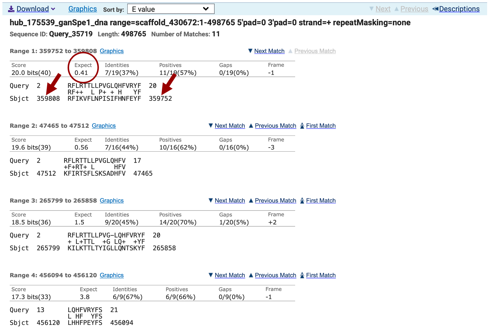
The “Alignments” section shows the alignments between the query and the subject ranked by E-value (Figure 15). Remember the query is the CDS sequence, and the subject is your translated project sequence. Note that none of the matches have coordinates on the subject line in the range we expect to find this CDS (somewhere around 151,000-151,500) based on the SPALN alignments tracks on the Genome Browser (Figure 3). We can conclude that none of these matches have any biological significance and probably this first CDS is not well conserved between N. vitripennis and Ganaspis sp.1.
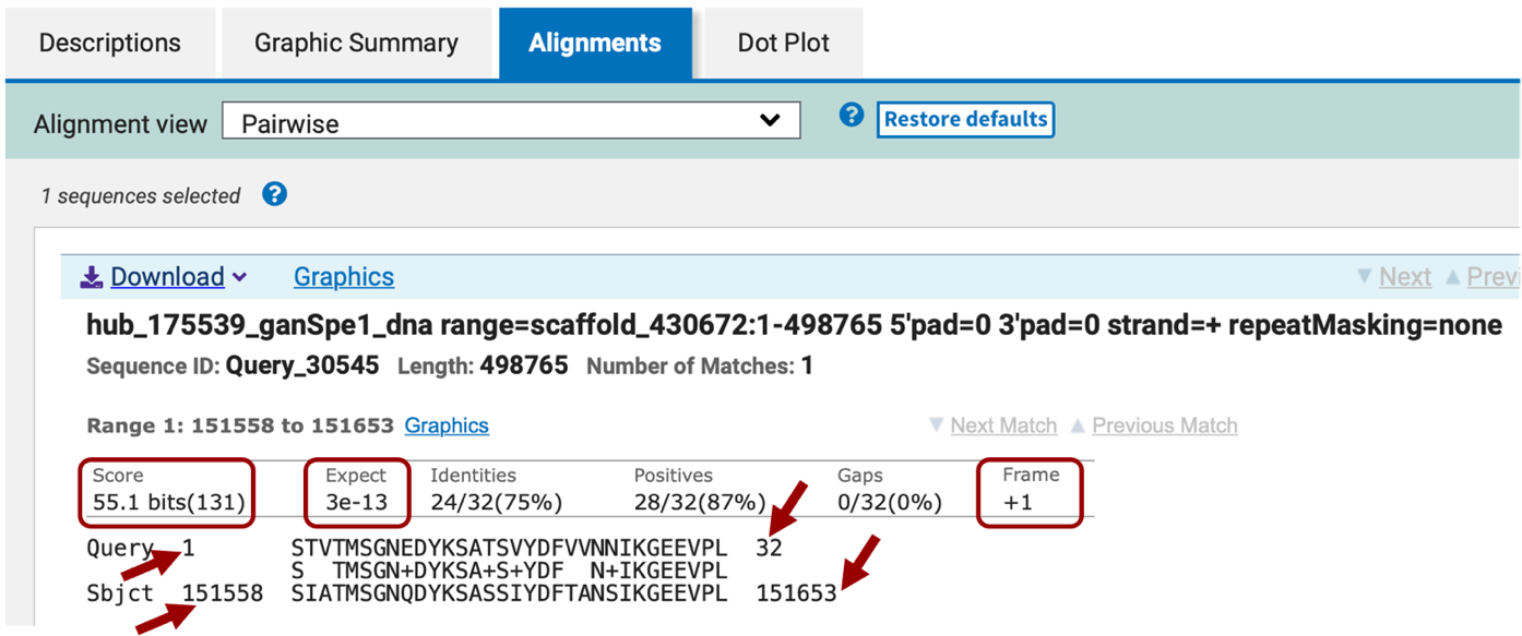
We will nevertheless continue searching for the other CDSs following the same protocol. Go to the Gene Record Finder tab and select the second CDS of LOC100677983 and paste it in the Query sequence box of the tblastn window. Keep all the parameters the same and click BLAST. In this case, the BLAST search returns three hits with Expect values less than 10. The most significant hit has a score value of 55.1 and an E-value of 3e-13 (Figure 16). This hit is listed first in the alignments section. The two other alignments produced have significantly lower scores and higher E-values. They also match coordinates in the scaffold that are not where we expect the ortholog to be.
Make a note of three items from this BLAST alignment result:
-
the subject coordinates where the CDS aligned to the scaffold sequence, in this case 151,558-151,653
-
the translated frame from your scaffold to which the amino acid sequence matches, in this case +1
-
Remember, any DNA fragment can be read in three frames on the plus (top) strand, and 3 frames in the minus (bottom) strand.
-
-
whether the alignment was full-length; in this case, the query length was 33 amino acids, and the BLAST alignment began at #1, and extended through #32, so the last amino acid was not aligned
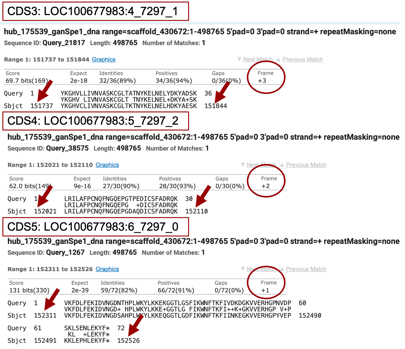
Repeating this process with the three other CDSs for isoform XP_008210670.1 identifies significant matches for these three CDSs (Figure 17).
Notice that the entire sequences of these last three CDSs aligned to the scaffold sequence, which indicates that the 3' end of the gene is more conserved than the 5' end. Also, this example illustrates the concept that it is recommended searching for sequence similarity using the largest CDS’s first to anchor the gene model (in this case CDS5 which is 72 amino acids long; CDS1 is just 21). A larger sequence has higher probability of finding some regions of similarity.
Map the Exact Coordinates of Each CDS
Once you have the approximate location of the CDSs you will return to the Genome Browser to map their exact start and end coordinates for each of them. In this case because the tblastn match for CDS1 is not statistically significant (E-value = 0.41), we will start with the second CDS.
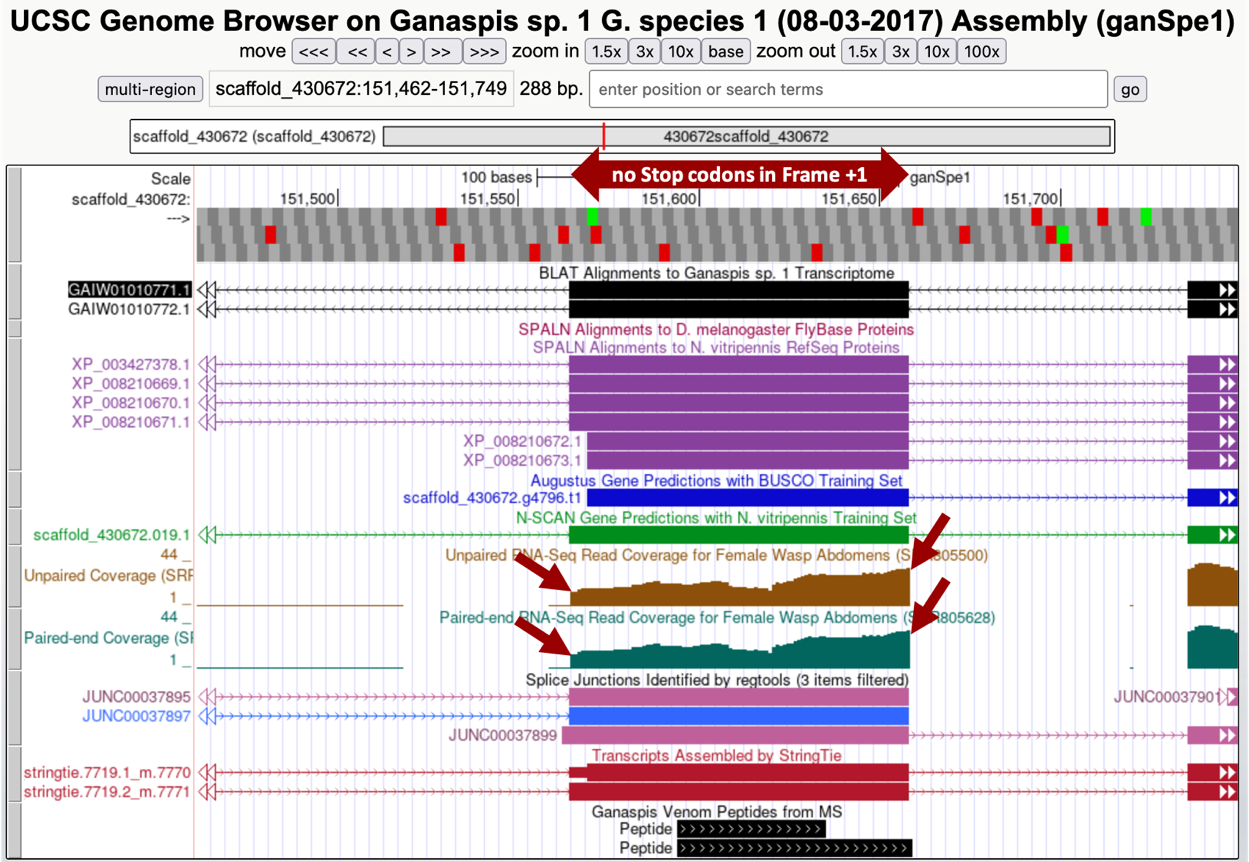
Recall that tblastn identified a match for CDS2 in frame +1 from 151,558-151,653 of the DNA assembly and begins with the amino acid sequence STV (query). Center your Genome Browser on scaffold_430672:151,558-151,653 in the search box, click on the “Search” button, then zoom out 3x. Your screen should look similar to that of Figure 18. Look at the Unpaired and Paired-end RNA-Seq Read Coverage tracks. These tracks were obtained by sequencing RNAs (mostly mature mRNAs) and the reads were mapped against the genome assembly. The more abundant the RNA, the more reads were produced and so the higher the peaks. Both of the displayed RNA-Seq tracks show peaks, indicating that this region is transcribed into RNA (red arrows on the Figure 18 mark the beginning and end of the RNA signal). Also, notice that for the region with good RNA-Seq coverage, only frame +1 shows an Open Reading Frame (ORF) — there are no stop codons (indicated by red boxes in the “Base Position” track) in this reading frame.
Determine the exact position of the beginning of the second CDS: LOC100677983:2_7297_2
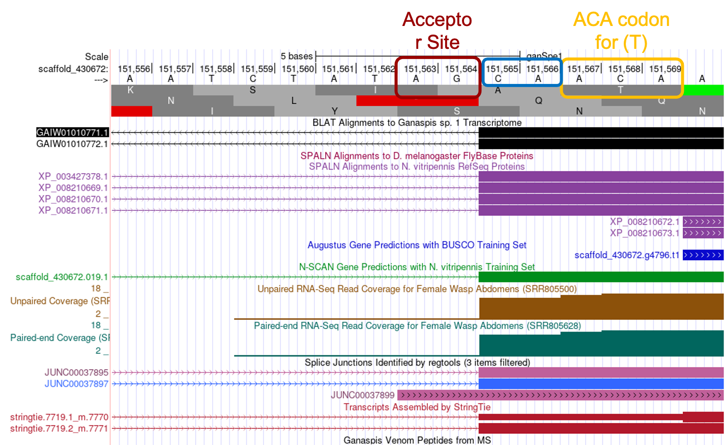
To determine the exact position of the beginning of the CDS, enter “scaffold_430672:151,556-151,570” in the search box, alternatively you can navigate to 151,558 and zoom out until you have about 15-20 nucleotides in view (Figure 19).
The RNA-Seq coverage starts to peak at 151,565, the nucleotide at that position is C. Right before this nucleotide, and still as part of the intron, you can observe the nucleotides AG, which are the consensus signal for the splice acceptor. Several other lines of evidence support the idea that the C at position 151,565 marks the beginning of the exon: (1) The StringTie assembly of transcripts, which builds transcript models by assembling the RNA-Seq reads using the genome sequence as reference, predicts two transcripts both of which have an intron-exon boundary at that position. (2) Similarly, the “G1 Transcriptome” track, which shows a BLAT alignment of a de novo assembled transcriptome with the genome sequence, also predicts an intron-exon boundary there. (3) The “Splice Junction” track, which tries to predict exon-intron boundaries based on RNA-Seq reads that span the introns, has two predictions “JUNC00037895” and “JUNC00037897” pointing to the same location. (4) As expected from our tblastn search using the individual N. vitripennis CDSs for the XP_008210670.1 isoform, which found a perfect alignment from amino acid T beginning of the CDS2 the “SPALN Alignment to N vitripennis RefSeq Proteins” track identifies four proteins that support the start site for the exon. In conclusion, the evidence supports annotating the C at position 151,565 as the start of the exon in frame +1. The tblastn alignment had tried to extend the homology past the exon/intron boundary, but as you see in Figure 16, from the first four amino acids only the S was aligned, and the best alignment starts with amino acid T.
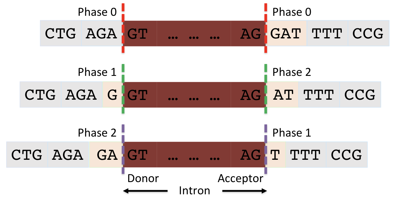
Before moving on to annotate the end of the CDS, there is one more piece of evidence we need to collect, namely the phase of the reading frame (to review splicing and the concept of phase, watch the Splicing and Phase video).
Phase depends on the reading frame of the CDS and is defined as the number of bases between the complete codon and the splice site.
-
Donor phase: number of bases between the end of the last complete codon and the splice donor site (GT/GC)
-
Acceptor phase: number of bases between the splice acceptor (AG) and the start of the first complete codon
For example, Figure 20 illustrates the three possible phases.
Applying this terminology to the annotation of the 5' end of the CDS2 (Figure 19), one sees there are two nucleotides (C and A) between the splice acceptor site (AG) and the first full amino acid of the CDS (T amino acid encoded by ACA). Therefore, the beginning of the 2nd CDS is in phase 2 for frame +1.
Determine the exact position of the end of the second CDS: LOC100677983:2_7297_2
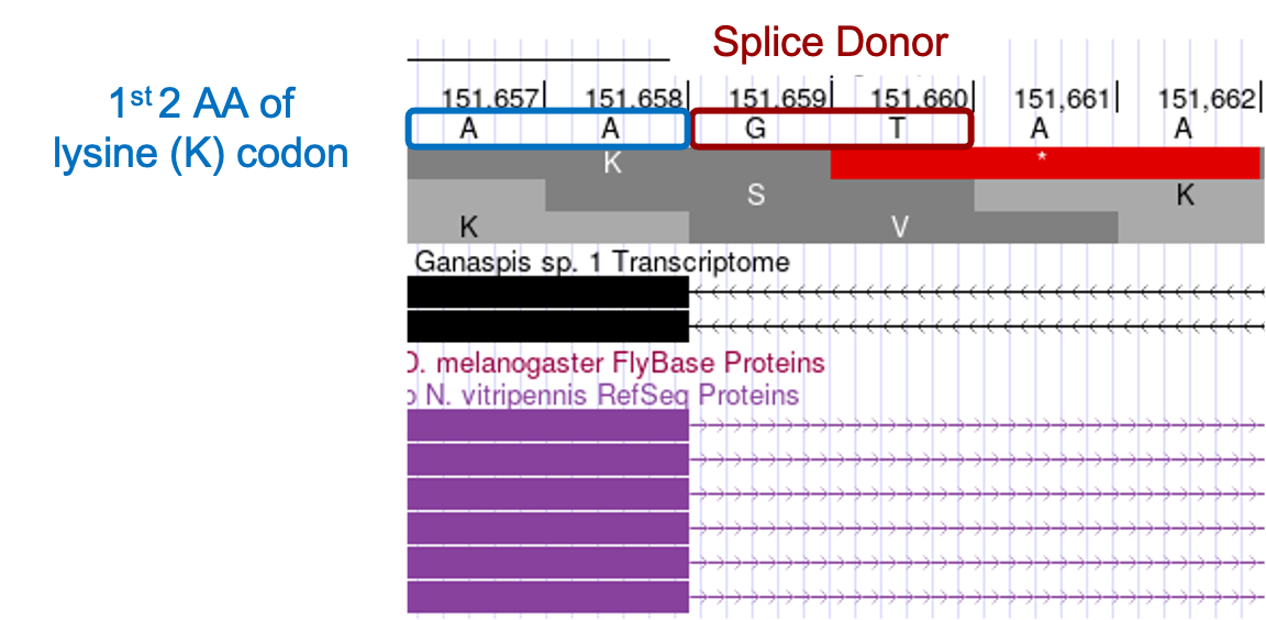
To determine the exact position of the 3' end of the CDS, enter “scaffold_430672:151,637-151,681” in the search box. The RNA-Seq coverage ends at the nucleotide A at position 151,658, and it is followed by the canonical splice donor GT. As with the start of the CDS, several lines of evidence support the A at 151,658 marking the end of the CDS.
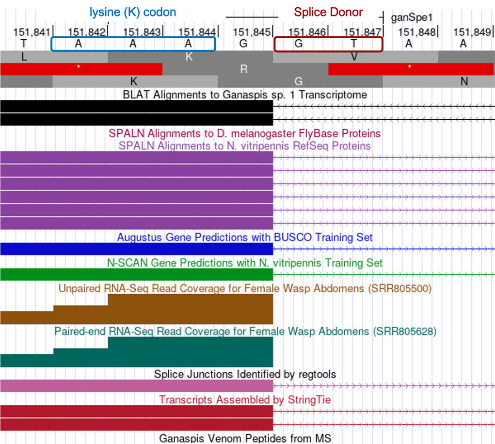
Examining the 3' end of the CDS, one sees that the splice donor site (GT) generates a phase 2 donor by interrupting the lysine codon between the 2nd and 3rd nucleotides (Figure 21). As a result, the start of the next exon should be in phase 1 in order to reconstitute the reading frame.
Determine the exact position of the start of the third CDS: LOC100677983:4_7297_1
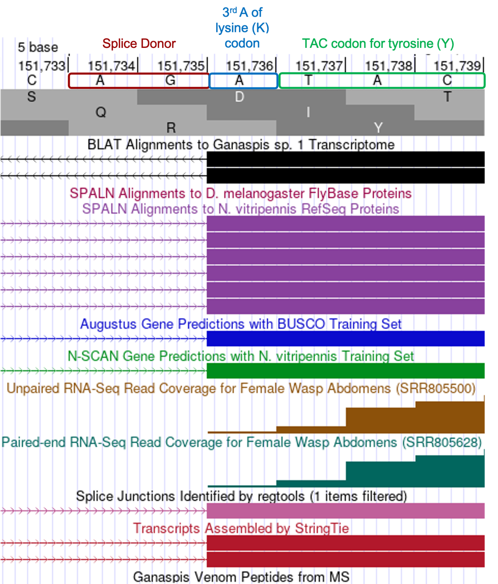
The coordinates of next several CDSs can be determined using the same procedure as just described for the 2nd CDS. First, our tblastn alignment for the third exon LOC100677983:4_7297_1 (Figure 17), begins at 151,737 and ends at 151,844 in reading frame +3. To observe all three translated frames, center your Genome Browser on scaffold_430672:151,737-151,844 in the search box, click on the “Search” button, then zoom out 3x. Consistent with the tblastn data, we see there are no stop codons in frame +3, whereas both +1 and +2 frames do contain stop codons in this region. Now, navigate to the beginning of the CDS by zooming around coordinate 151,737 so you see about 6 nucleotides (Figure 22). The RNA-Seq coverage starts at 151,736, the nucleotide at that position is A, which is preceded by nucleotides AG, which are the consensus signal for the splice acceptor. The tblastn alignment suggests the CDS of this exon should start with the amino acids YKG, and we see the codon for Y begins at 151,737. As a result, there is a single A nucleotide (151,736) between the splice acceptor and the first full codon (Y), making this a phase 1 acceptor. This A nucleotide together with two AA nucleotides at the end of the previous CDS generates the AAA codon, which codes for lysine (Figure 22).
Determine the exact position of the end of the third CDS: LOC100677983:4_7297_1
Turning your attention to the 3' end of the exon, the tblastn alignment ends at 151,844 in reading frame +3, with the last two conserved amino acids being SK. Center your browser on that location to identify the exact end of the exon. The RNA-Seq evidence supports the end of the exon occurring at G residue located at 151,845 with a splice donor (GT) immediately following. This position is also supported by BLAT alignments, SPALN alignments to N. vitripennis, RNA-Seq junctions and StringTie data. Examining the phase arrangement, we find the intron is inserted after the 1st nucleotide (G) of a codon, i.e., phase 1 intron (Figure 23).
Determine the exact position of the start of the fourth CDS: LOC100677983:5_7297_2
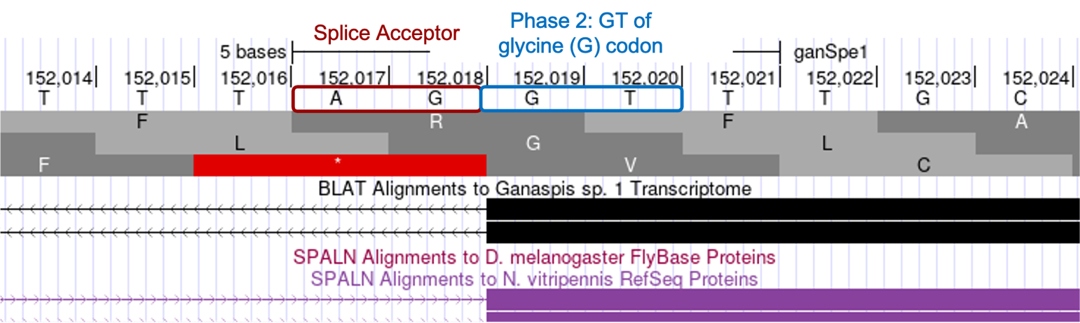
The tblastn alignment for the 4th exon LOC100677983:5_7297_2 (Figure 17), begins at 152,021 and ends at 152,110 in reading frame +2. Consistent with the tblastn data, we see there are no stop codons in frame +2, whereas both the +1 and +3 frames do contain stop codons in this region. The RNA-Seq coverage starts at 152,019, the nucleotide at that position is G, and is preceded by splice acceptor consensus nucleotides AG. The tblastn alignment suggests the CDS of this exon should start with the amino acids LRI, and we see the codon for L (TTG) begins at 152,021. Therefore, the GT residues at position 152,019-152,020 completes the glycine codon from the previous exon (GGT) — confirming this exon starts in phase 2 (Figure 24).
Determine the exact position of the end of the fourth CDS: LOC100677983:5_7297_2
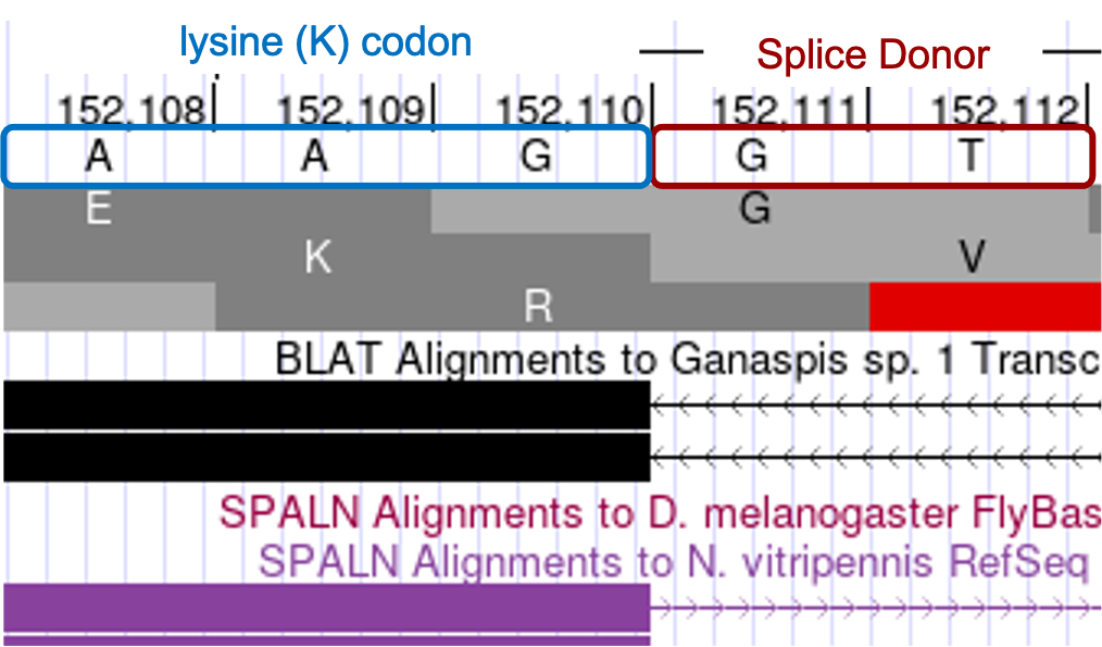
The tblastn alignment ends at 152,110 in reading frame +2, with the last two conserved amino acids being QK. Center your browser on that location to identify the exact end of the exon. The RNA-Seq evidence supports the end of the exon occurring at G residue located at 152,110 with a splice donor (GT) immediately following. This position is also supported by BLAT alignments, SPALN alignments to N. vitripennis, RNA-Seq junctions and StringTie data. Examining the phase arrangement, we find the intron is in phase 0, the codon terminates with a complete AAG lysine codon (Figure 25).
Determine the exact position of the start of the last CDS: LOC100677983:6_7297_0
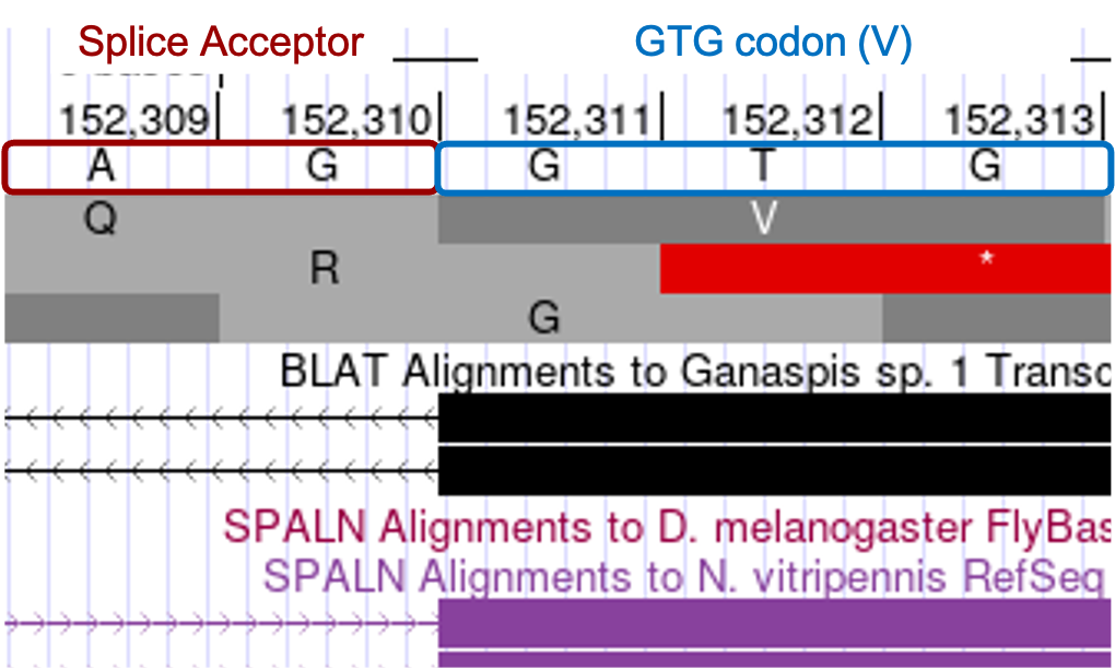
The tblastn alignment for the last CDS LOC100677983:6_7297_0 (Figure 17), begins at the 152,311 and ends at 152,526 in reading frame +1. Consistent with the tblastn data, we see there are no stop codons in frame +1, whereas both the +2 and +3 frames do contain stop codons in this region. The RNA-Seq coverage starts at 152,311, the nucleotide at that position is G, and is preceded by splice acceptor consensus nucleotides AG. The tblastn alignment suggests the CDS of this exon should start with the amino acids VKF, and we see the codon for V (GTG) begins at 152,311 in phase 0 (Figure 26).
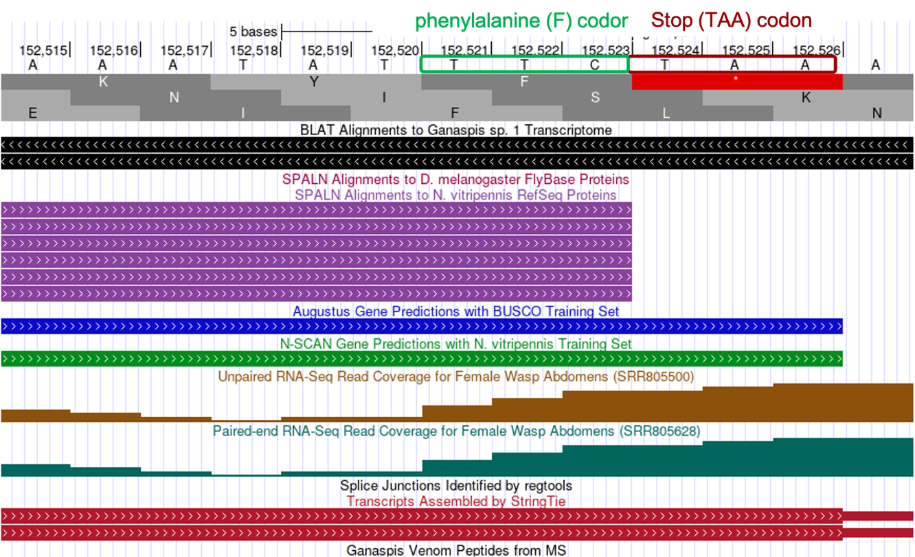
Determine the exact position of the end of the last CDS: LOC100677983:6_7297_0, and location of the stop codon.
The tblastn alignment for the last CDS LOC100677983:6_7297_0 (Figure 17) ends at 152,526 in reading frame +1 and the last three aligned amino acids are KYF. The codon (TTC) at positions 152,521-152,523 for the terminal Phenylalanine (F) amino acid is immediately followed by a stop codon (TAA) at 152,524-152,526. Therefore, we would annotate the end of the last CDS to be at 152,523 and the stop codon to be at 152,524-152,526 (Figure 27).
Determine the exact position of the end of the first CDS: LOC100677983:1_7297_0
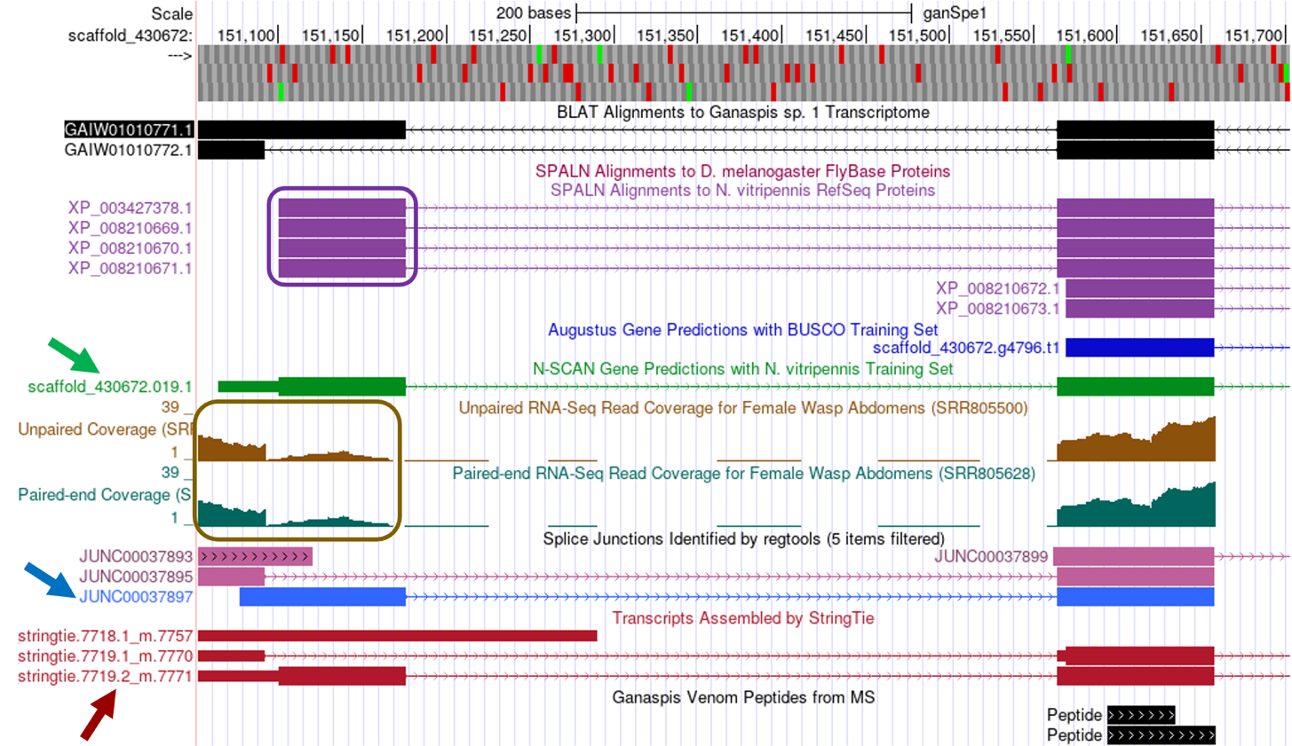
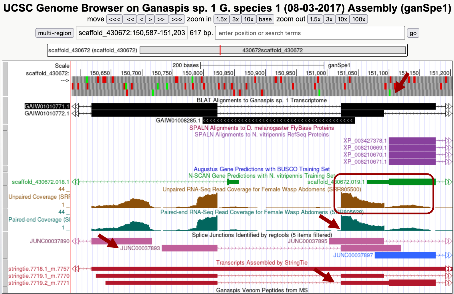
At this point, we have multiple lines of evidence supporting the start and end positions for the last four CDS exons for LOC100677983, but we’re unable to locate the 1st CDS by tblastn. [The best tblastn match to the 1st CDS is located at 359,808-359,752 in frame -1 (Figure 15), which is inconsistent with the locations and orientations of the other CDS exons.] We expect the 1st CDS to be located upstream of the 2nd CDS, which begins at 151,565 (Figure 19). To determine the best location for the 1st CDS, we should survey the region upstream of the 2nd CDS for evidence that points to the presence of another CDS. Examining the region scaffold_430672:151,050-151,680 (Figure 28), one sees five lines of evidence that potentially predict the position of the 1st CDS:
-
four SPALN alignments to N. vitripennis (purple box)
-
N-SCAN gene prediction overlaps with SPALN alignments (green arrow)
-
one regtools splice junction prediction (JUNC00037897, blue arrow) links the 2nd CDS to the region identified by SPALN alignments
-
one StringTie prediction (7719.2_m.7771, red arrow) links the beginning of CDS2 to the same region
-
RNA-Seq data (brown box) also overlaps the SPALN alignments.
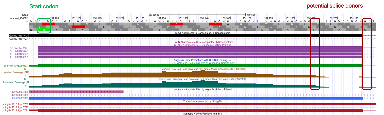
Zooming into this region, scaffold_430672:151,099-151,179, considering the SPALN alignments: (1) reading frame +3 begins with a Methionine codon (coordinates 151,101-151,103), (2) frame +3 is uninterrupted by stop codons, (3) two potential splice donor sites are identified towards the end of the SPALN alignment (GT-151,165 and GT-151,177), the first of which is supported by unpaired and paired-end RNA-Seq read coverage data, the latter supported by the splice junction data and is consistent with the end of the SPALN alignment (Figure 29).
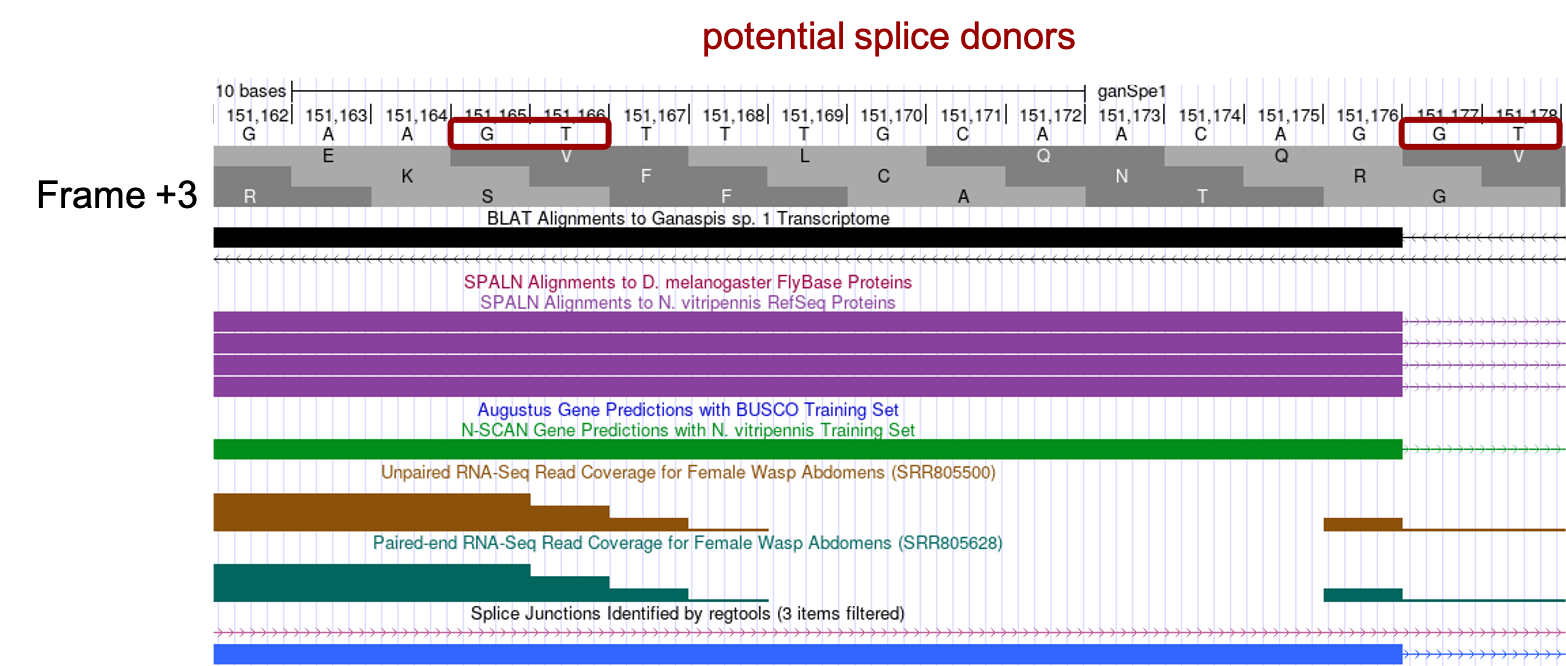
We know the start of the 2nd CDS was in phase 2, therefore we predict the end of the 1st CDS will be in phase 1. Examining the end of the 1st CDS (Figure 30) we see that both potential splice donors would generate a phase 1 in frame +3, however as can be seen on Figure 28 and Figure 29, most of the evidence (SPALN alignments to N. vitripennis, splice junction JUNC00037897, StringTie prediction 7719.2_m.7771, N-SCAN gene prediction) supports the end of the CDS at 151,176. Thus, we would annotate the 1st CDS coordinates to be 151,101-151,176.
Annotate the 5' UTR and 3' UTRs
Because the 5' and 3' UTRs are not usually conserved between these two wasps species, you will not use blastn searches to locate these. Instead, you will rely on RNA-Seq data tracks (i.e., Paired and Unpaired Coverage, Splice Junctions, and StringTie Transcripts predictions).
Annotate the 5' UTR
You expect to have untranslated RNA upstream of CDS1, either as part of the same exon or as an upstream exon separated by an intron. In the Genome Browser, zoom in the area to the left of CDS1 including it (Figure 31). Three lines of evidence indicate that CDS1 is contained within a larger exon that extends to the left of CDS1: RNA-Seq coverage, Splice Junction prediction JUNC00037890, and a StringTie prediction 7719.2_m.7771. The methionine of the CDS1 is indicated with a blue arrow, and RNA-Seq coverage can be observed upstream of it (red box). Consistent with this data, 7719.2_m.7771 StringTie prediction shows a block with a thin box (untranslated RNA) and a thick box (translated). The Splice Junction prediction JUNC00037890 also shows that this exon would be connected to another upstream exon.
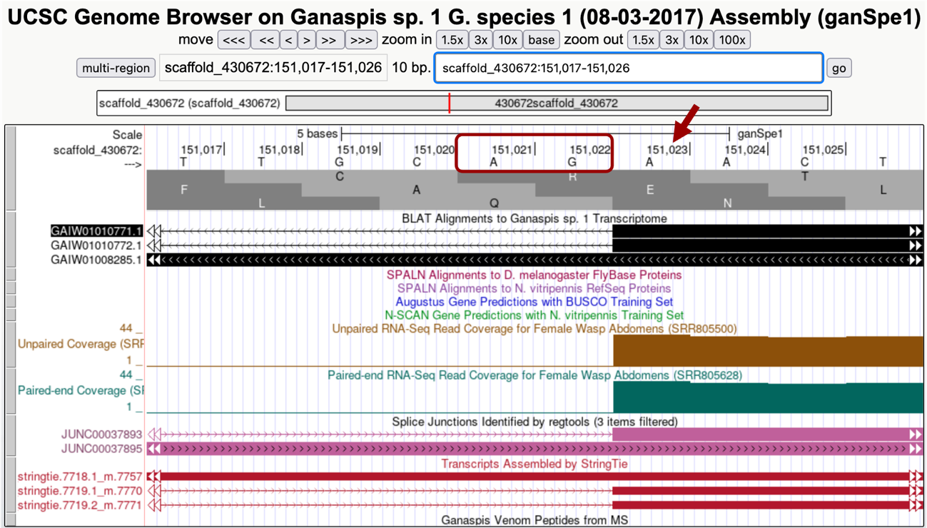
Zooming into the region at the 5' of this exon in your browser so it shows about 10 nucleotides, a splice acceptor, AG, can be seen at 151,021-151,022 and thus we would annotate the beginning of this exon at 151,023 (Figure 32). Since we already determined that CDS1 was 151,101-151,176 (Figure 28 and Figure 30). The entire exon coordinates are 151,023-151,176, of which 151,023 to 151,100 nucleotides are untranslated.
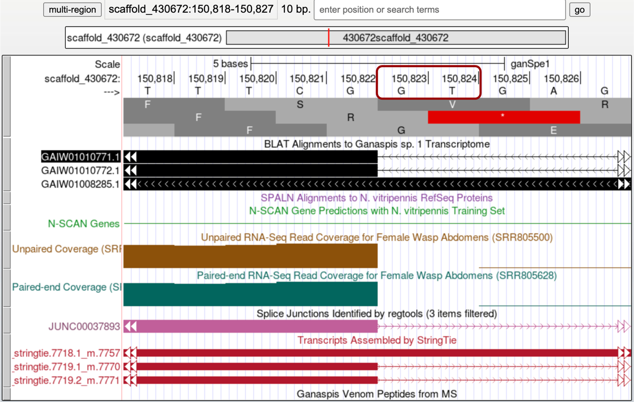
As indicated above Splice Junction prediction JUNC00037890 links this exon to another exon upstream. Zooming in at the end of that exon so about 10bp are in view, shows a GT donor site at 150,823-150,824, putting the end of that exon at 150,822 (Figure 33).
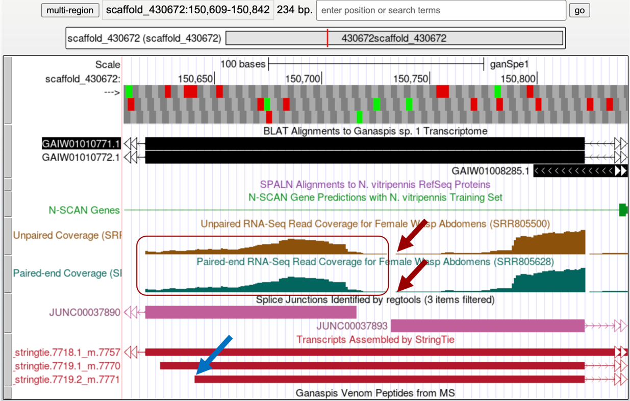
Judging by the RNA-Seq coverage profile this appears to be the first exon of the gene. To annotate the beginning of this transcript, you can observe the RNA-Seq coverage and the StringTie transcripts tracks (Figure 34). According to the RNA-Seq coverage, RNA reads seem to go down at 150,735 (red arrows) to come up again on the left. This region appears to be the 5' area of two divergent genes, the one we are annotating going right and another gene going to the left. The left RNA-Seq histogram (box in Figure 34) may be totally or partially contributed by the left gene (notice the sharp ending of the RNA-Seq coverage on the left end indicative of an exon/intron boundary).
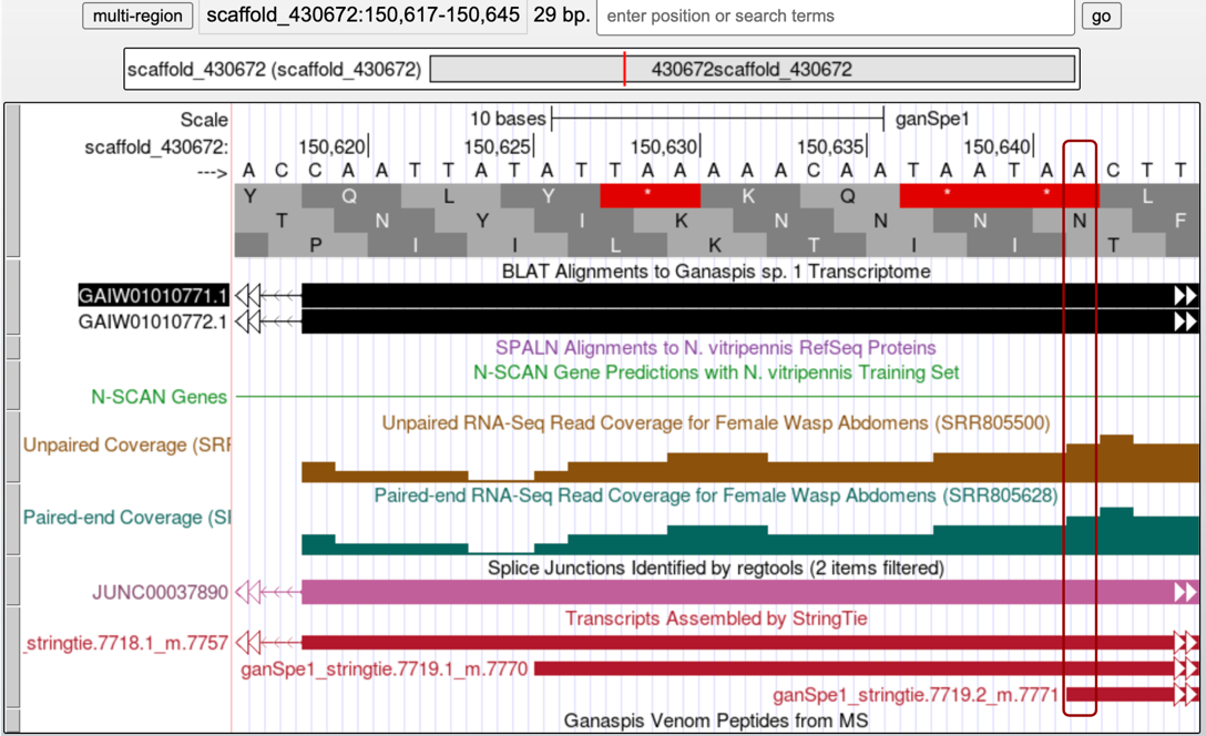
However, the StringTie prediction that we have been following (7719.2_m7771, blue arrow in Figure 34) puts the beginning of the transcript somewhere upstream of the region with no RNA-Seq coverage, at 150,642 (Figure 35). Considering that it is hard to ascertain what RNA-Seq reads may be coming from the gene on the left versus the gene on the right, we would go with the StringTie prediction and annotate this first exon coordinates as 150,642-150,822.
Annotate the 3' UTR
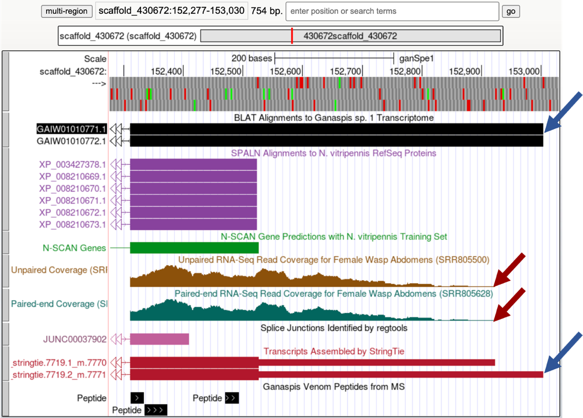
You expect to find untranslated RNA immediately after the protein’s stop codon. We mapped that at 152,524-152,526 (Figure 27). On the Genome Browser zoom in around the last CDS and include the area to the right as shown in Figure 36 (~152,277-153,030). Judging by the RNA-Seq profile, the last CDS appears to be part of the final exon: RNA-Seq coverage gradually winds down, there are no splice junction predictions going into the right, and the StringTie predictions also end in that area (Figure 36).
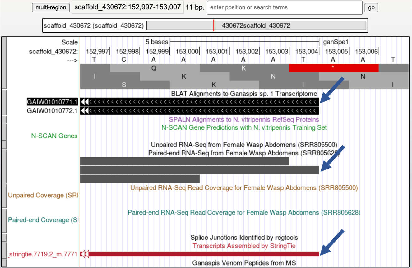
Although the RNA-Seq coverage appears to go down at 152,923 (red arrows, you will need to zoom in to determine the exact coordinate) and it is in agreement with the StringTie transcript prediction 7719.1_m7770, both the GAIW01010771.1 transcriptome assembly and the StringTie transcript prediction 7719.2_m.7771 point to the end of the transcript being at 153,004. On the Genome Browser, set the Pair-ended RNA-Seq BAM and Unpaired RNA-Seq BAM tracks to pack. Zoom in close to the end of the StringTie prediction 7719.1_7771 as shown in Figure 37. The Pair-ended RNA-Seq reads also end at 153,004. Thus, we would annotate the last exon at 152,311-153,004, where the 152,311-152,526 corresponds to the last CDS including the stop codon, and the 152,527-153,004 is the 3' UTR.
Validate Hypothesized Gene Model using Gene Model Checker
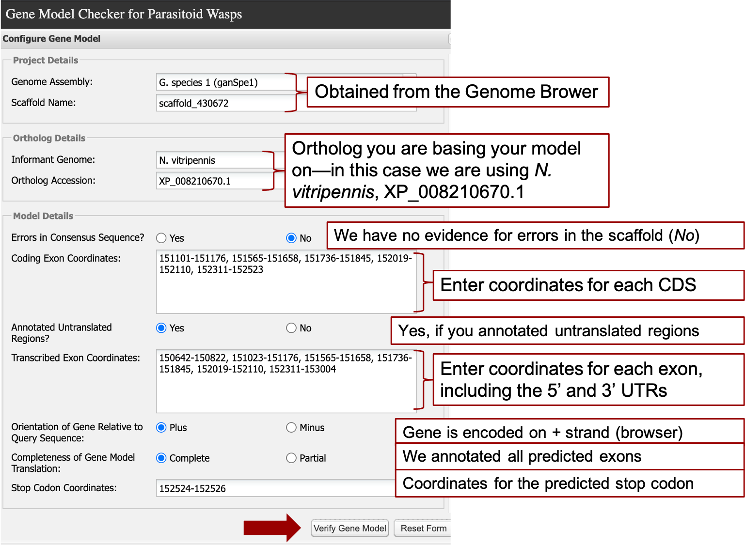
Now that you have predicted the exact coordinates for each CDS for one isoform, we will use the Gene Model Checker for Parasitoid Wasps to validate the predicted gene model.
The required information for Gene Model Checker for this walkthrough is shown below (Figure 38).
The last CDS should not include the stop coordinates, these are entered in the last field “Stop Codon Coordinates” which auto-fills when you click on it based on the last reported coordinates of the last exon. Note that the transcribed exon coordinates will have the exons that comprise the first and last CDS. For example, CDS1 (151,101-151,176) is included in the second transcribed exon (151,023-151,176), and the last CDS (152,311-152,523) is included in the last exon (152,311-153,004). Selecting “Verify Gene Model” at the bottom carries out an in-silico splicing reaction using the ortholog and coordinates you provided.
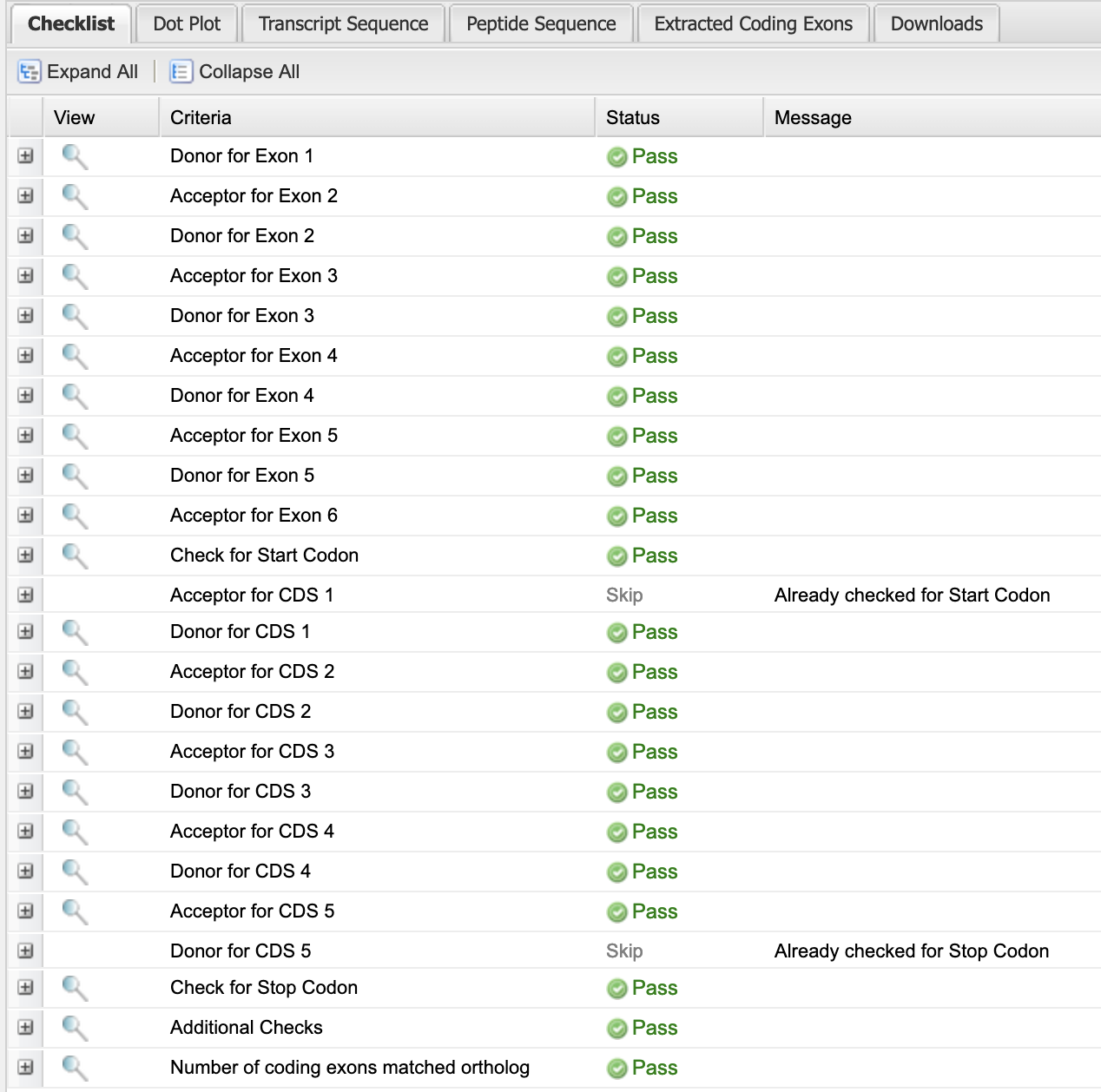
If the coordinates provided result in no splicing errors, the resulting checklist would show Pass for the Start codon, all splice donor / acceptor pairs, and the stop codon (Figure 39).
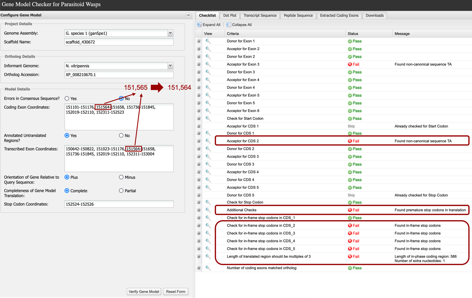
In many cases, errors that result in a “Fail” in the Gene Model Checker are the result of an “off-by-one” error in specifying a splice donor or acceptor. For example, if we change the acceptor site for CDS2 (and transcribed exon #3) from 151,565 to 151,564 we will obtain the result shown below (Figure 40). If you click on the “+” in the left column next to “Acceptor for CDS 2”, the sequence context of the acceptor site defined by the coordinates is shown. Here we see that one nucleotide change in the coordinates for the acceptor site for CDS 2 resulted in a non-canonical splice acceptor (TA) error. In addition, this one nucleotide error results in in-frame stop codons downstream (Figure 40, bottom red box).
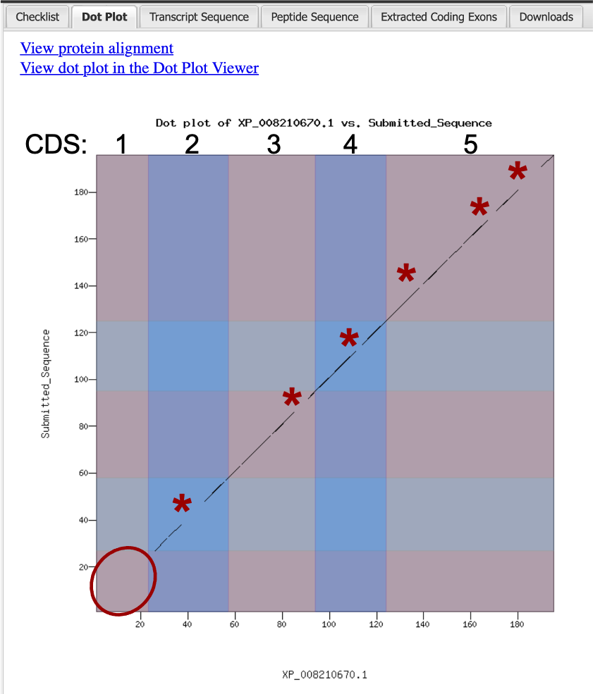
Dot Plot
The Gene Model Checker provides additional data that is useful in assessing the validity of your predicted gene model. The Dot Plot feature compares the amino acid sequence derived from the coordinates you provided against the N. vitripennis ortholog (XP_008210670.1). If the amino acid sequences are identical, the dot plot should result in a diagonal line. The results of the predictions made for the G. species 1 (08-03-2017) Assembly (ganSpe1) homolog of N. vitripennis XP_008210670.1 are shown below (Figure 41). Note that the Dot Plot shows no alignment for CDS1, which indicates that the sequences for this CDS have diverged in the two species.
Download Files
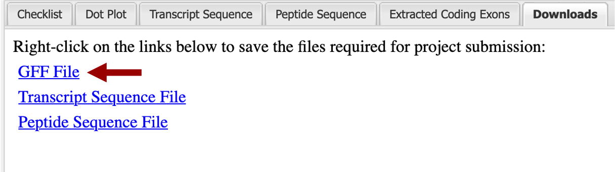
On the right side of the “Gene Model Checker” window click on the “Downloads” tab. The next window will have a list of three options “GFF File”, “Transcript Sequence File”, and “Peptide Sequence File” (Figure 42). You will need to save all three types. Start by right clicking on the “GFF File” link.
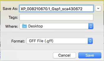
Download the GFF File and change the file name while preserving the “.gff” file extension. It is recommended that you follow a standard naming system: isoform name of reference genome_annotating species name_scaffold. In our example that name would be XP_008210670_Gsp1_sca430672.
Depending on which web browser you’re using, you will have a pop-up window similar to the one shown in Figure 43. Save that file in a folder within your computer. Under format, verify that the file type is GFF, by default it will have .gff extension. Repeat the process for the Transcript and Peptide Sequence Files. You can use the same file name; they will have different extensions.
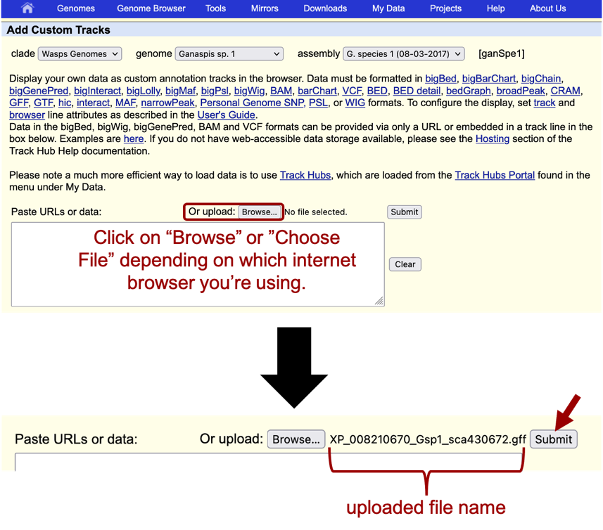
Add Custom Track to the Browser
In order to see your gene model in the context of the other evidence tracks on the browser, you will need to upload the GFF File. Go to the Genome Browser window and click on the “Add custom tracks” button found under the viewer window. On the window that opens up, click on the “Choose File” or “Browse” button to the right of the “Paste URLs or data” section and navigate to the .gff file you saved in your computer. In this example, select the file “XP_008210670_Gsp1_sca430672.gff” and then click on “Submit” (Figure 44).
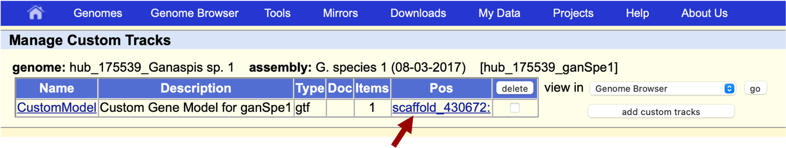
On the next window, click the link with the project name, “scaffold_430672” in our example (Figure 45).
The name of the model can be customized by clicking “CustomModel” and entering the desired name. We will leave the default option here.
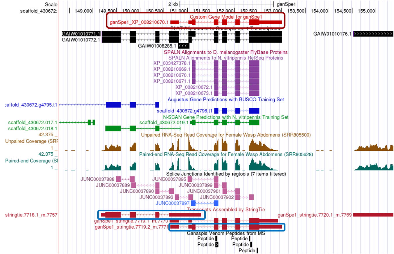
The next screen will have a new track “Custom Gene Model for ganSpe1” (red box) with your gene model centered around the coordinates you annotated. You can click zoom out 3x to have a view of the general area (Figure 46).
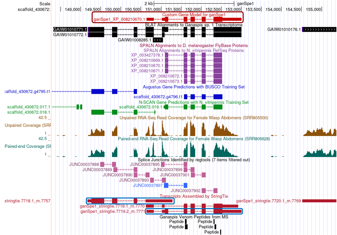
Under this zoomed-out view, it can be appreciated that the de novo transcriptome GAIW01010771.1 prediction is probably bringing together two separate genes. Both Augustus and N-SCAN predict a gene on the left part of the region. Also, StringTie predictions fall into two separate sections (blue boxes).
-
For the purpose of the submission of your project, you will need to take a screenshot of the Genome Browser with your gene model on it.
Bibliography
-
[Mortimer et al., 2013] Mortimer NT, Goecks J, Kacsoh BZ, Mobley JA, Bowersock GJ, Taylor J, Schlenke TA. Parasitoid wasp venom SERCA regulates Drosophila calcium levels and inhibits cellular immunity. Proc Natl Acad Sci U S A. 2013 Jun 4;110(23):9427-32. doi: 10.1073/pnas.1222351110.
-
[Goecks et al., 2013] Goecks J, Mortimer NT, Mobley JA, Bowersock GJ, Taylor J, Schlenke TA. Integrative approach reveals composition of endoparasitoid wasp venoms. PLoS One. 2013 May 23;8(5):e64125. doi: 10.1371/journal.pone.0064125.