Prerequisites
-
Understanding Eukaryotic Genes (UEG) Modules 1, 4, 5, & 6
-
An Introduction to NCBI BLAST or Sequence Similarity Introduction
Resources & Tools
-
All links for this walkthrough, including the recommended prerequisites listed above, can be found on the Pathways Project page of the GEP website (thegep.org/pathways).
Introduction
The Pathways Project is focused on annotating genes found in well characterized signaling and metabolic pathways across the Drosophila genus. The current focus is on the insulin signaling pathway which is well conserved across animals and critical to growth and metabolic homeostasis. The long-term goal of the Pathways Project is to analyze how the regulatory regions of genes evolve in the context of their positions within a network. For a general project overview, see the 6-minute video.
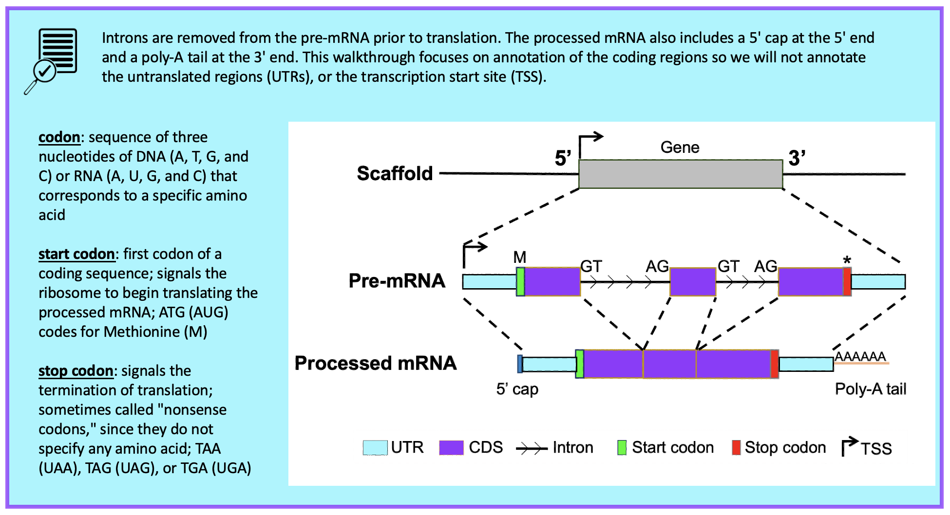
This walkthrough illustrates how to apply the Genomics Education Partnership's (GEP) annotation strategy, for the Pathways Project, to construct a gene model for the Ras homolog enriched in brain (Rheb) gene (target gene) in Drosophila yakuba (target species). This walkthrough focuses on annotation of the coding regions only, so we won’t annotate the untranslated regions (UTRs), nor the transcription start site (TSS).
It is important to note that the Rheb gene in D. yakuba is a relatively straightforward annotation project in comparison to what your own project might be. Some of the steps in this walkthrough might appear to be excessive, but keep in mind that you will potentially have a more complex project, so it is important to follow this protocol as it will equip you with most of what you will need should you encounter complexities. We recommend you follow the parts in the order they are presented, and then refer to parts when needed for your own project. Note that the figures have been configured to fit this document while still maintaining readability; therefore, your screen may differ slightly. Commas have been included with most coordinates to improve readability, but you do not have to enter them in the Genome Browser (navigation will work the same with or without commas). Terms located in the Glossary are red and bolded typically the first time they are mentioned in the walkthrough and not necessarily every time they’re mentioned. |
|
Part 1: Examine genomic neighborhood surrounding target gene in D. melanogaster
|
Figure 1. Review of content from UEG Module 1
|

-
On the following “FlyBase Protein-Coding Genes” page, click on “Rheb-RA at chr3R:5568921-5570491” (Figure 3).
 Figure 3. Since both Rheb-RA and Rheb-RB span the same coordinates, it doesn’t matter which of the two we select (Figure 4). Navigate to the Rheb gene in D. melanogaster by clicking on Rheb-RA (arrow).
 Figure 4. For Your Information — Isoforms with differing coordinates
-
Because the Genome Browser remembers our previous track display settings, click on “default tracks” in the display controls below the Genome Browser image (Figure 5).
 Figure 5. The “default tracks” button quickly removes any display changes you previously made and returns to the defaults.
 Figure 6. Review of content from UEG Module 1. There are three major sections of the Genome Browser—a set of navigation controls, the Genome Browser image, and a set of track display controls.
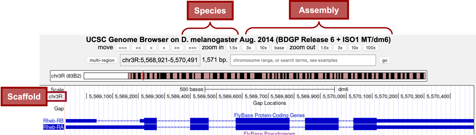
In the “FlyBase Protein-Coding Genes” track, we should now see the gene structure for the two isoforms (Figure 6) of the Rheb gene (i.e., Rheb-RA and Rheb-RB). Notice that Rheb is on the “chr3R” scaffold (Figure 7).

-
Zoom out until you can see the nearest two genes on each side of Rheb.
We are now viewing the genomic neighborhood of the Rheb gene in D. melanogaster (i.e., region of the scaffold containing Rheb (target gene) and its neighboring two closest upstream genes and two closest downstream genes; Figure 9).

Now we need to draw a sketch of the genomic neighborhood of Rheb in D. melanogaster (Figure 11). To do so, we must identify the direction of transcription for each gene by zooming in on an intron (or exon) of each gene.
-
Start by zooming in on an intron (or exon) of Rheb.
-
Since the arrows within the introns of Rheb point to the right, in our sketch we need to draw an arrow pointing to the right and label it Rheb.
-
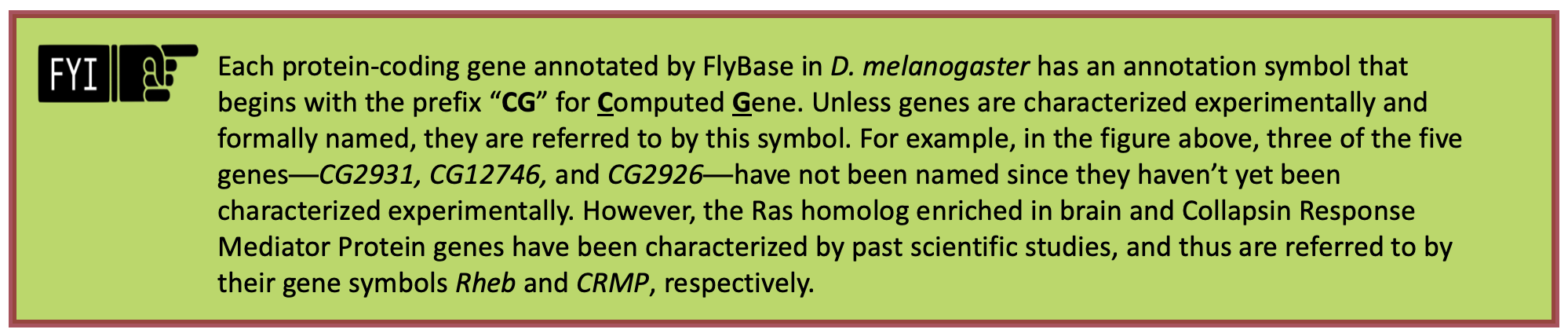
Repeat Steps 9-10 for the two closest genes on both sides of Rheb (i.e., CG12746, CG2931, CRMP, and CG2926).
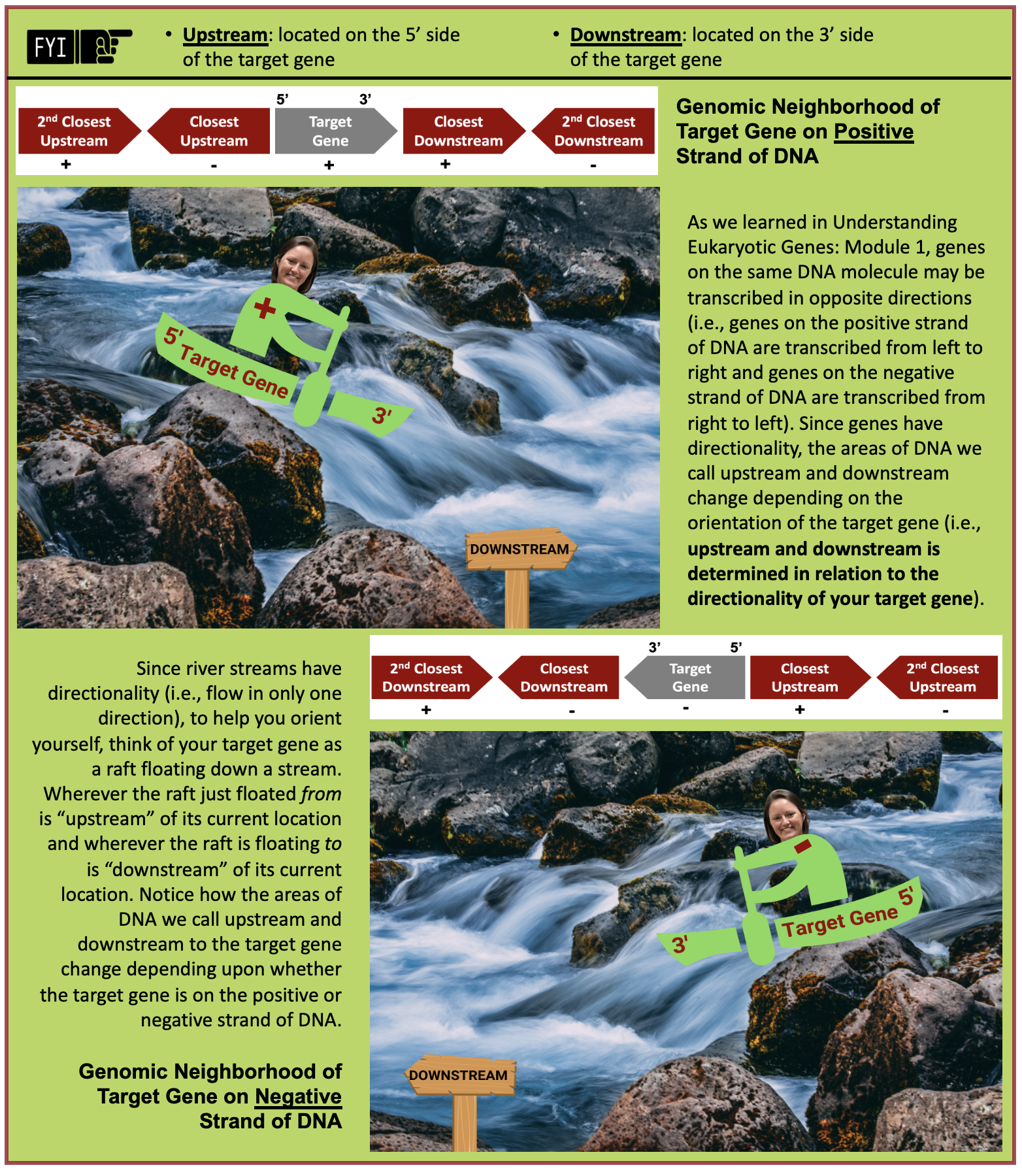
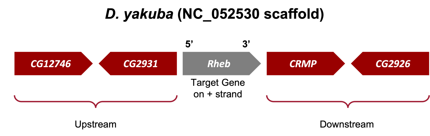
The arrows within the introns of Rheb point to the right; therefore, we know Rheb is transcribed from left to right and located on the positive strand of DNA in D. melanogaster. Since Rheb is our target gene (i.e., gene we are annotating), the two closest genes on its 5' side are considered upstream and the two closest genes on its 3' side are considered downstream (Figure 12).
-
The two closest upstream genes to Rheb in D. melanogaster are CG2931 and CG12746.
-
The two closest downstream genes to Rheb in D. melanogaster are CRMP and CG2926.

Part 2: Identify genomic location of ortholog in target species
Now that we’ve examined the genomic neighborhood of our target gene, Rheb, in D. melanogaster, we need to identify the location of Rheb in our target species D. yakuba.
Part 2.1: Retrieve protein sequence of target gene in D. melanogaster
-
In the “FlyBase Protein-Coding Genes” track, click on “Rheb-RA” (Figure 13).

-
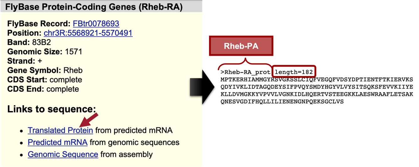
Under the “Links to sequence” heading, click on the “Translated Protein” link (Figure 14, left).
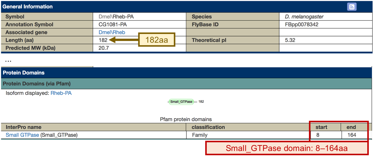
We are now viewing the sequence for the 182 amino acids in the translated protein of Rheb-RA in D. melanogaster (Figure 14, right).
-
Copy the entire sequence (including the header) so we can use it in our tblastn search.
Part 2.2: Perform a BLAST search of D. melanogaster protein against the target species' genome
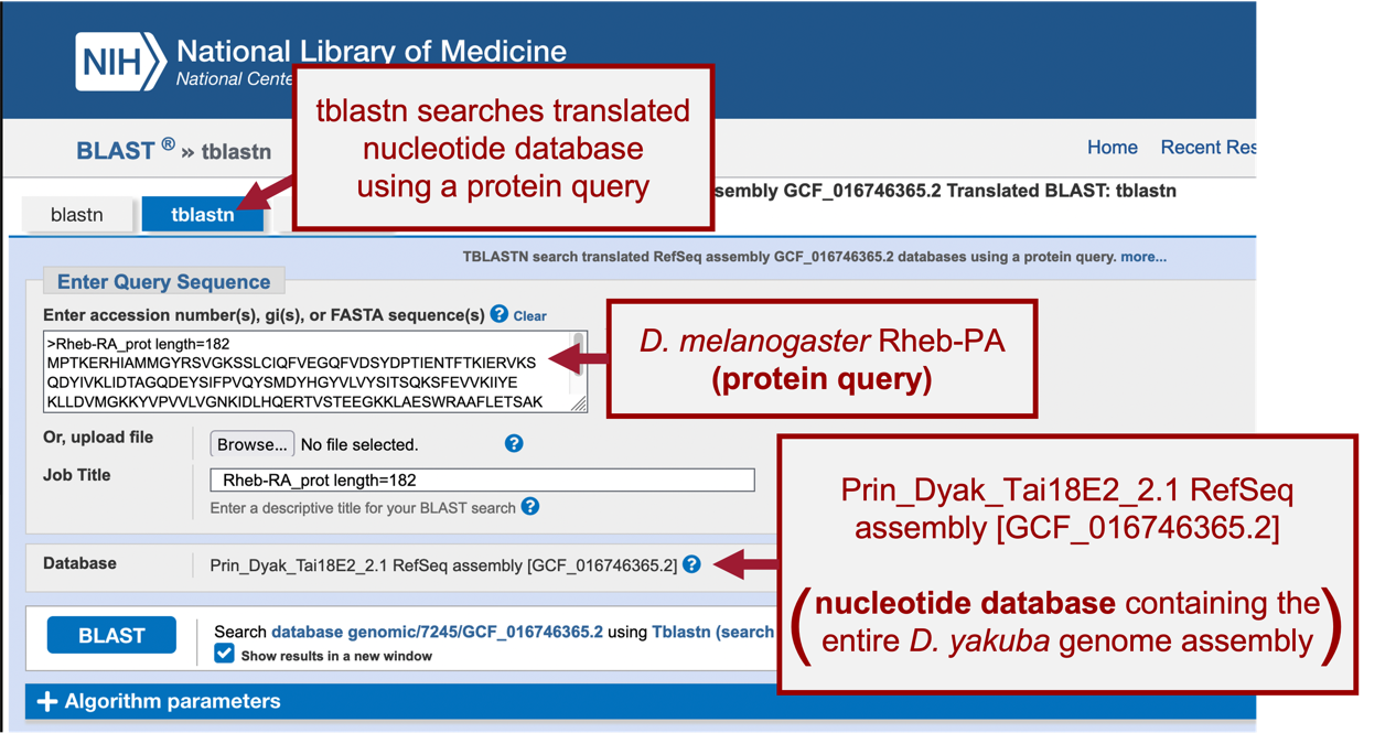
In Part 2.1, we retrieved the protein sequence for Rheb-PA in D. melanogaster. Now we need to perform a BLAST search (Figure 16) of Rheb-PA against the entire D. yakuba genome assembly.
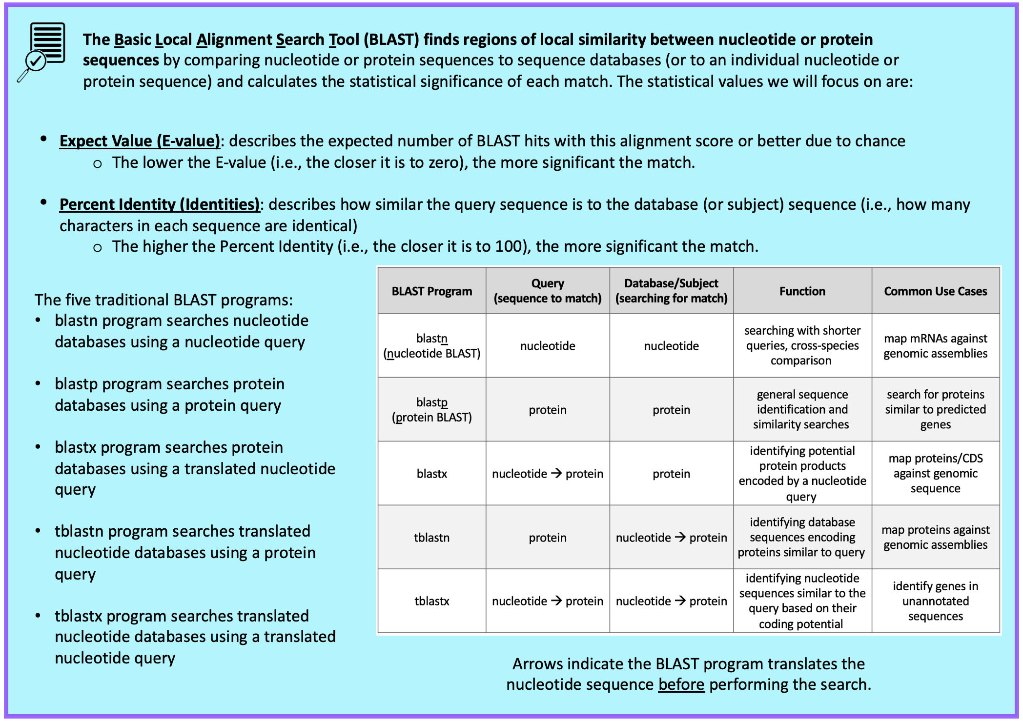
Since we are looking for the orthologous region of Rheb in D. yakuba, we want to use BLAST to search the entire genome of D. yakuba to identify regions of local similarity with the protein sequence of Rheb in D. melanogaster we obtained in Part 2.1. In other words, we need to perform a BLAST search of our Rheb protein sequence from D. melanogaster against the entire genome of D. yakuba to narrow down the possible regions where the Rheb ortholog could be in D. yakuba.
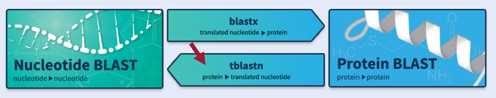
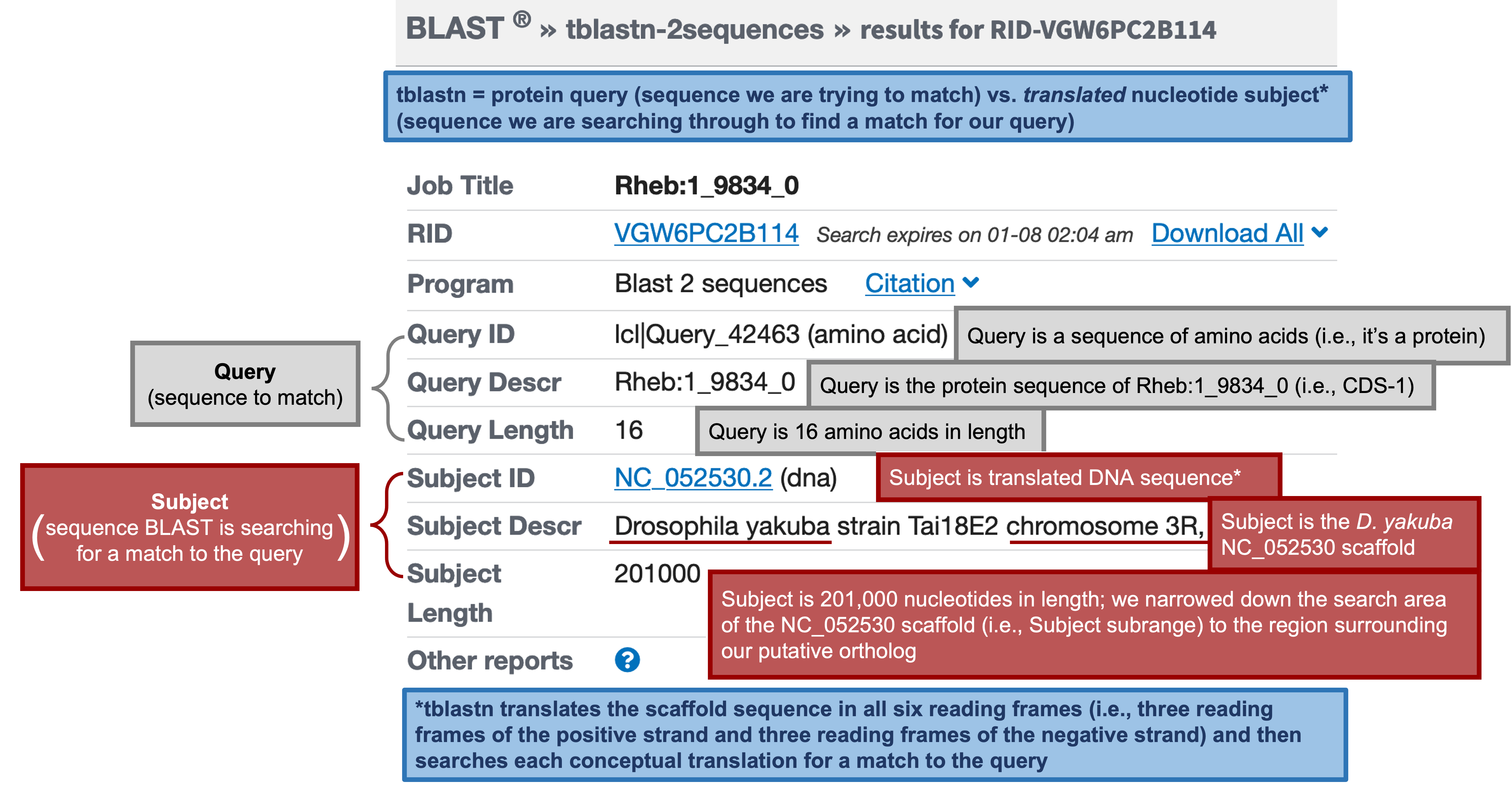
For this BLAST search, we will use the tblastn program to search the translated nucleotide database of our target species, D. yakuba, using the protein sequence of Rheb in D. melanogaster as our query.
-
Query: sequence we are looking to match (i.e., protein sequence of Rheb in D. melanogaster)
-
Database (Subject): collection of sequences we are searching for matches (BLAST will translate the entire genome of D. yakuba before searching for a match to the Rheb-PA sequence from D. melanogaster)
-
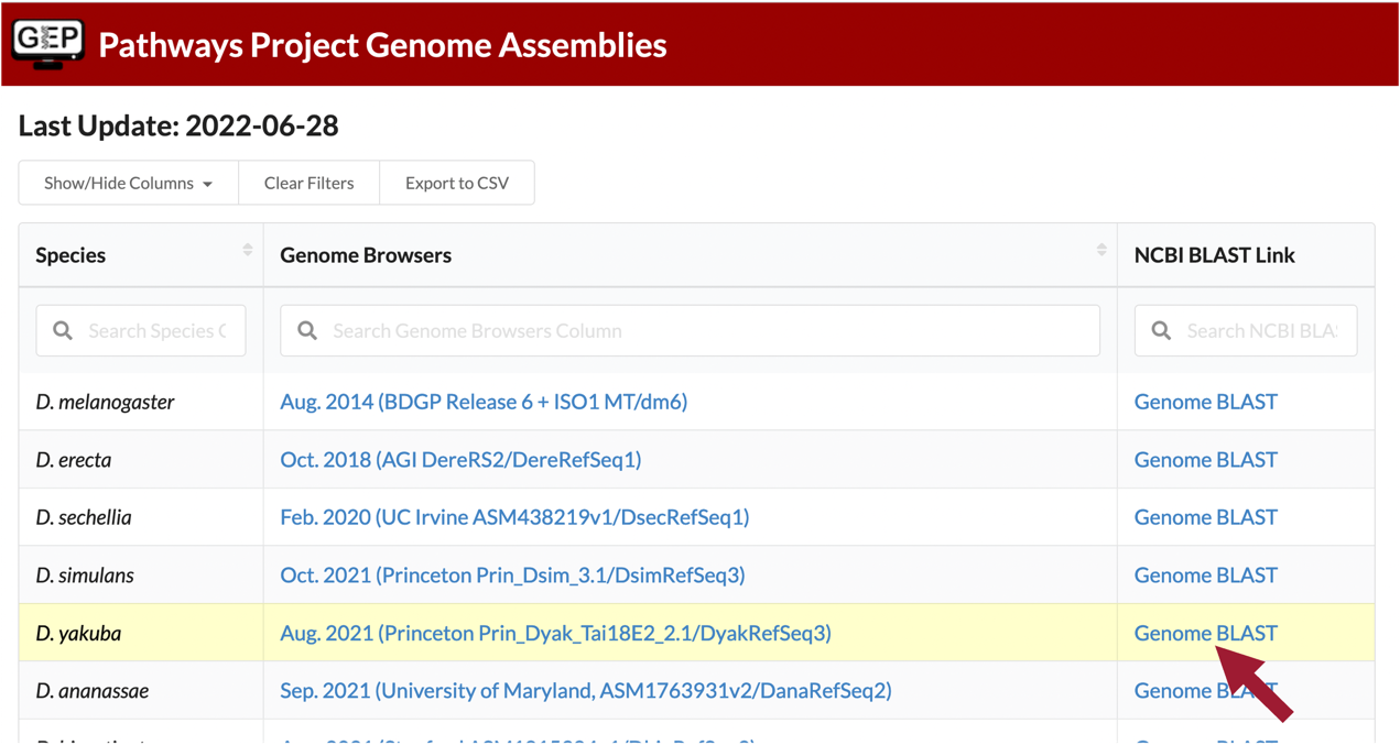
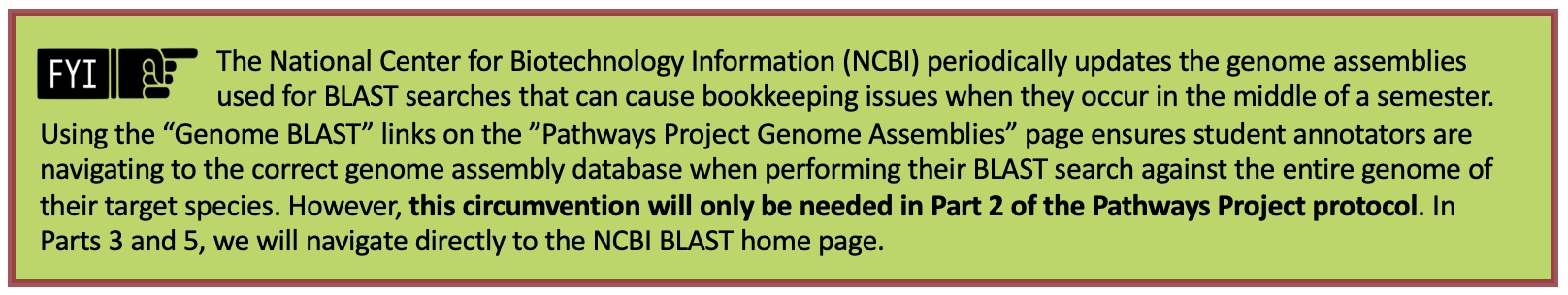
Navigate to the Pathways Project Genome Assemblies page.
-
Click on the “Genome BLAST” link for D. yakuba (Figure 17).

Here we are selecting the entire genome of D. yakuba (~148 million bases) as the database for our tblastn search (Figure 18).
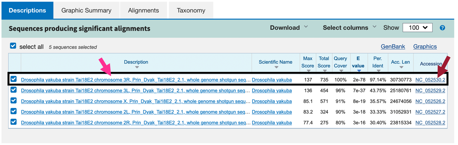
When performing a search, BLAST may return any number of matches (often referred to as “hits”) for regions of local similarity between our query sequence and database; however, each hit is not necessarily statistically significant. BLAST provides statistical scores to help us determine which alignments between the two sequences are statistically significant and which are spurious (i.e., likely occurred by chance and, therefore, are not evidence of real biological conservation). If BLAST returns multiple good hits (i.e., more than one match with a low E-value and a high sequence identity), we will need to investigate them all further to determine the most likely ortholog.
Our tblastn search found five regions within the translated D. yakuba genome that show similarities with the protein sequence of Rheb in D. melanogaster (Figure 21); however, only one of these is a good hit (Drosophila yakuba strain Tai18E2 chromosome 3R, Prin_Dyak_Tai18E2_2.1, whole genome shotgun sequence; sequence identity: 97.14% and E-value: 2e-78[1]). The second hit has a much higher E-value (7e-37) and much lower percent identity (43.75%), and this pattern of increasingly lower quality matches continues through the other three matches. Therefore, we will continue our analysis based on the hypothesis that the putative ortholog of Rheb-PA in D. yakuba is in the scaffold of chromosome 3R.
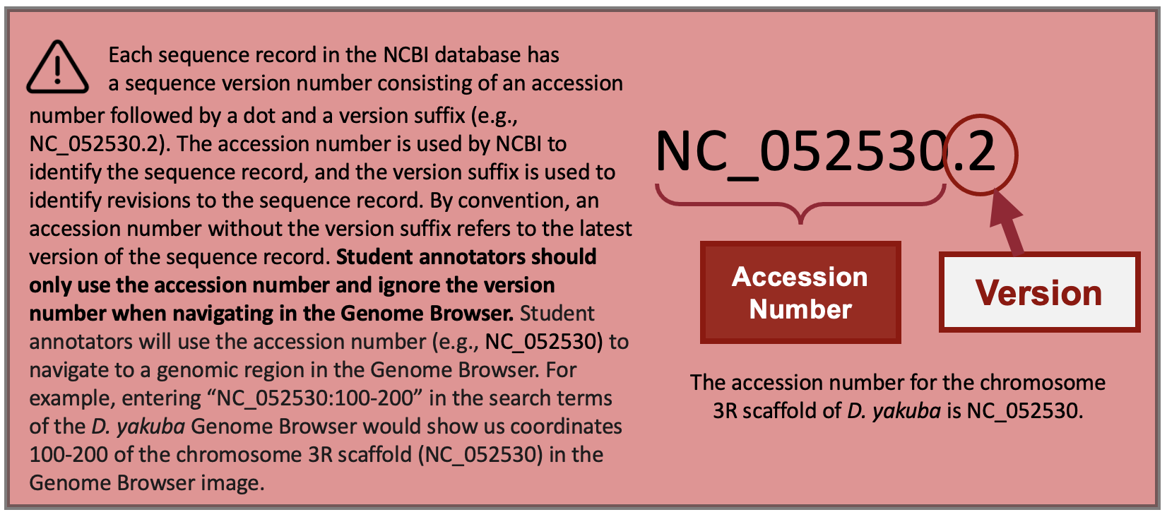
Notice that each of the genome regions of our five hits has a unique accession number (Figure 20).
The accession number for the chromosome 3R scaffold in D. yakuba is NC_052530 (Figure 21, red arrow).
Part 2.3: Summarize tblastn results for protein on target species' scaffold
-
Click on the “Drosophila yakuba strain Tai18E2 chromosome 3R, Prin_Dyak_Tai18E2_2.1, whole genome shotgun sequence” link in the “Description” column to navigate to the alignment (Figure 21, left arrow).
-
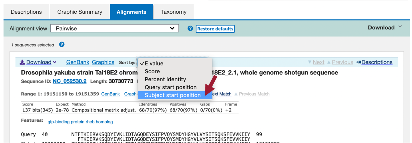
In the blue toolbar for the BLAST hit, select the “Subject start position” option from the drop-down menu of the “Sort by” field to order the matches based on the start coordinates on D. yakuba NC_052530 scaffold in ascending order (Figure 23).
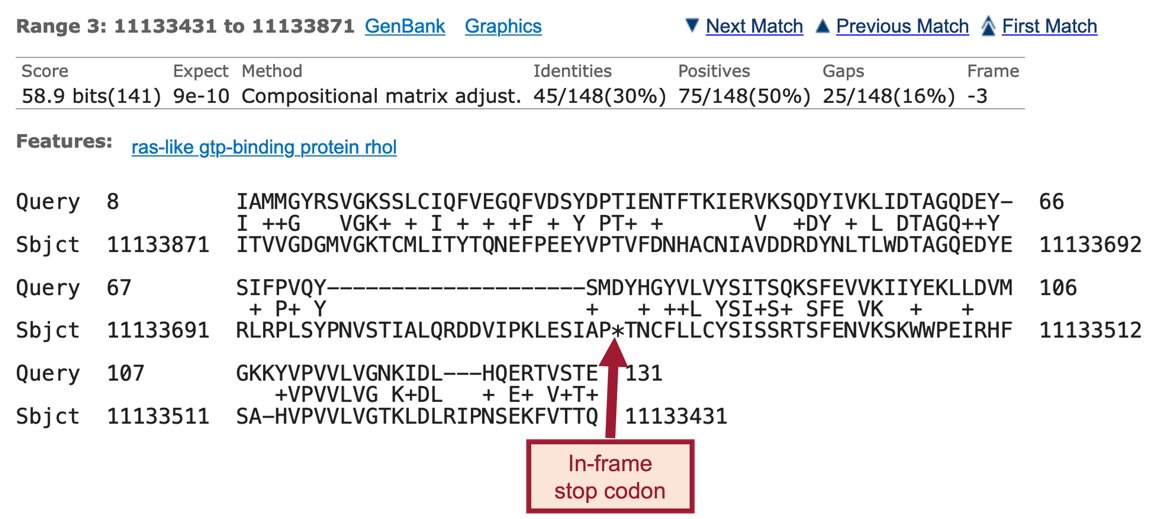
We should now see 7 ranges listed in ascending order of the subject start position (coordinate). Each range corresponds to a contiguous portion of the subject sequence (D. yakuba genome) that shows significant sequence similarity (i.e., matches) with a portion of the query sequence (D. melanogaster Rheb-PA). Here, the 7 ranges show matches between Rheb-PA in D. melanogaster (Query) and a range of coordinates from the NC_052530 scaffold in D. yakuba (Sbjct). For example, Range 1 shows a match between Rheb-PA in D. melanogaster (Query: 6 – 44) and coordinates 11,148,568 – 11,148,431 of NC_052530 scaffold in D. yakuba when translated in Frame -3. Range 1 has an E-value (Expect) of 0.002 and a sequence identity of 46% (Figure 24, green boxes).
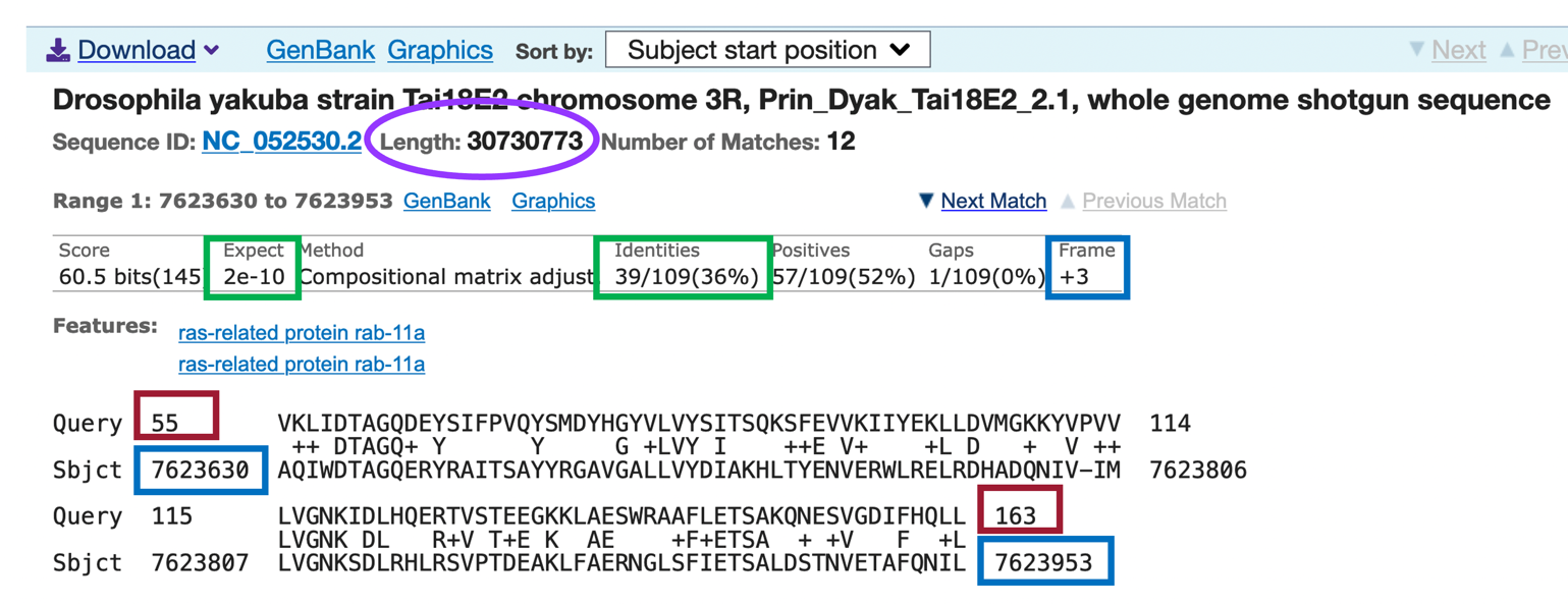
Since the NC_052530 scaffold in D. yakuba is 30,730,773 base pairs (bp) long (Figure 24, purple circle), it is possible we will have some ranges (i.e., alignment matches or hits) that don’t correspond to our ortholog; therefore, we need to examine each match more closely.
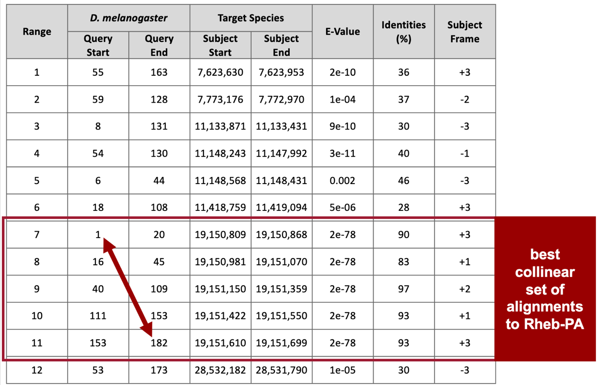
Remember that we are looking for matches with low E-values and high sequence identities, and there are five matches (ranges 3 – 7) that fit these criteria (E-value of 2e-78 and sequence identities that range from 83% to 97%). These five alignment matches are also collinear and appear on the same strand of DNA (+ Frame) (Figure 25).
The best collinear set of alignments to Rheb-PA is located at 19,150,809 – 19,151,699 on the NC_052530 scaffold of the D. yakuba genome assembly and the five alignment matches cover all 182 amino acids of Rheb-PA (Figure 25, arrow). Therefore, we will continue our analysis based on the hypothesis that the putative ortholog of Rheb-PA is located at approximately 19,150,809 – 19,151,699 on the NC_052530 scaffold of the D. yakuba genome assembly.
Part 3: Examine genomic neighborhood of putative ortholog in target species
In Part 1, we sketched the genomic neighborhood of Rheb in D. melanogaster. Here we will examine the genomic neighborhood of Rheb in D. yakuba (Figure 26) and then compare the order and orientation of these genes to what we found in D. melanogaster.
Based on parsimony, the genes surrounding Rheb in D. yakuba should be identical or very similar in sequence to the genes in the genomic neighborhood of Rheb in D. melanogaster. Additionally, the neighboring genes should also match in orientation (look at the direction of transcription of the neighboring genes; this is called local synteny). Since Rheb and CG2926 are on the positive and negative strand, respectively, in D. melanogaster, these two genes should also be on different strands in D. yakuba.

Part 3.1: Examine evidence for a protein-coding gene in region surrounding the tblastn alignment in the target species
-
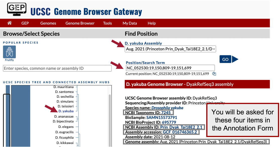
Navigate to the Genome Browser Gateway page.
-
Click on “D. yakuba” in the “UCSC Species Tree and Connected Assembly Hubs” table.
-
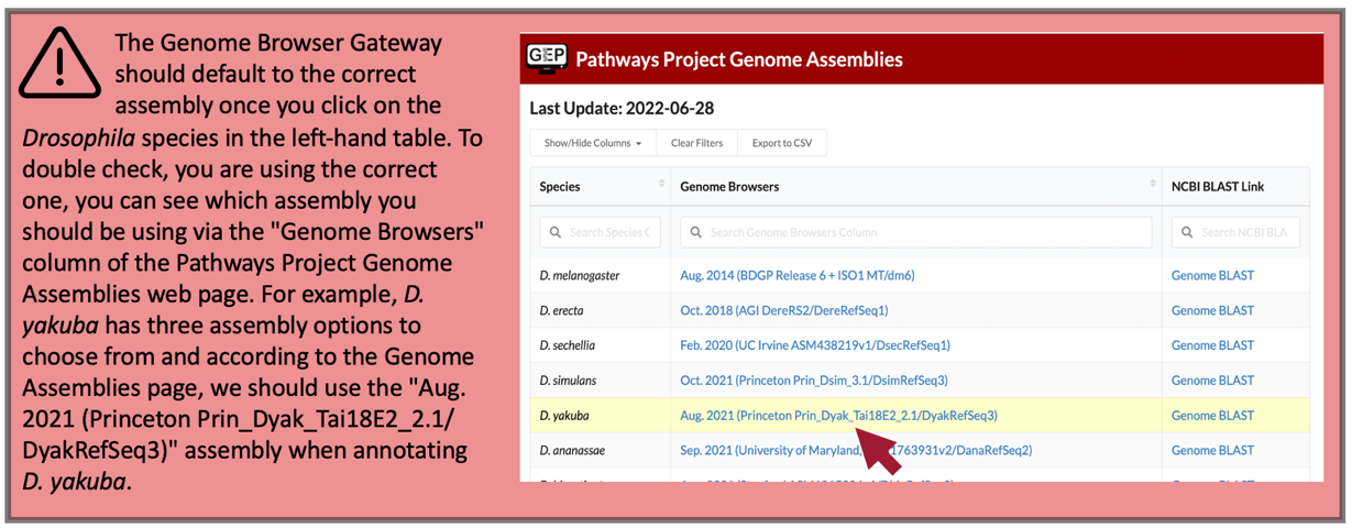
Under the “D. yakuba Assembly” field, confirm that “Aug. 2021 (Princeton Prin_Dyak_Tai18E2_2.1/DyakRefSeq3)” is selected (Figure 27).
-
In Part 2, we determined the putative ortholog of Rheb-PA is located at approximately 19,150,809 – 19,151,699 on the NC_052530 scaffold of the D. yakuba genome assembly. Enter “NC_052530:19,150,809-19,151,699” under the “Position/Search Term” field to examine this region.
-
Click on the “GO” button (Figure 28).
-
In the list of buttons below the Genome Browser image, click on “default tracks” (Figure 5).
-
Zoom out 3x.
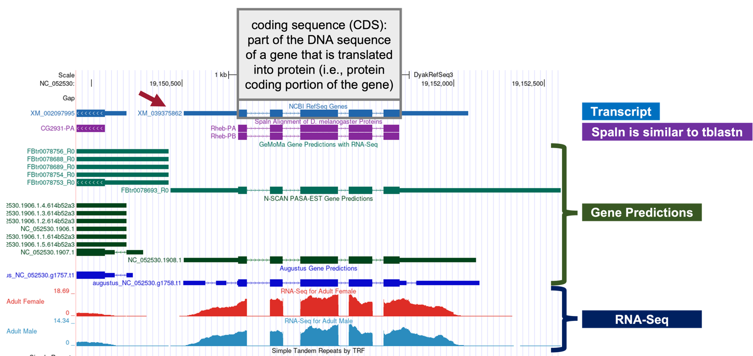
In the Genome Browser image, we should now see the following tracks (Figure 29):
-
NCBI RefSeq Genes
-
Spaln Alignment of D. melanogaster Proteins
-
Gene Prediction Tracks (Figure 30):
-
GeMoMa Gene Predictions with RNA-Seq
-
N-SCAN PASA-EST Gene Predictions
-
Augustus Gene Predictions
-
-
Aggregated RNA-Seq Coverage
Looking at the NCBI RefSeq Genes track, we notice that the alignment for the coding regions of the D. yakuba RefSeq transcript XM_039375862 against the NC_052530 scaffold of D. yakuba line up with the Spaln alignment to the D. melanogaster proteins Rheb-PA and Rheb-PB. Furthermore, the coding portions of the five alignment blocks are in congruence with the placements of the five coding exons (CDS’s) predicted by GeMoMa, N-SCAN, and Augustus.
According to the RefSeq transcript XM_039375862 (Figure 29, red arrow), the putative (probable) ortholog of Rheb-PA is located at NC_052530:19,150,510-19,152,080 in D. yakuba and the region spanning NC_052530:19,150,809-19,151,702, within the putative ortholog, corresponds to the alignment to the coding region of the RefSeq transcript.
Part 3.2: Use synteny to gather additional evidence for the ortholog assignment
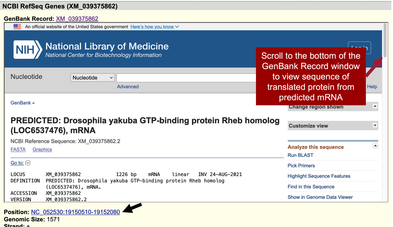
Notice the position of XM_039375862 is “NC_052530:19,150,510-19,152,080” (Figure 31, black arrow).
-
In the “Item Details” page, click on the “XM_039375862” link next to the “GenBank Record” label to view the GenBank record in a new window (Figure 31, top red arrow). Scroll to the bottom of the GenBank Record window to the “"translation"” sequence within the “CDS” section (Figure 32, rectangle).
We are now viewing the computationally predicted protein sequence of the putative ortholog to Rheb-PA in D. yakuba.
-
Copy the accession number for the translated protein sequence (Figure 32, arrow).
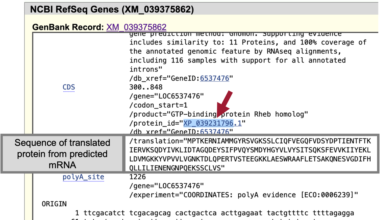
When we run BLAST for this protein, we can enter the accession number “XP_039231796” and the program will use the translated protein sequence shown in the grey box in Figure 32.
|
|
We recommend using the accession number instead of the actual sequence (i.e., MPTKERNIAMM…) to avoid formatting errors. |
-
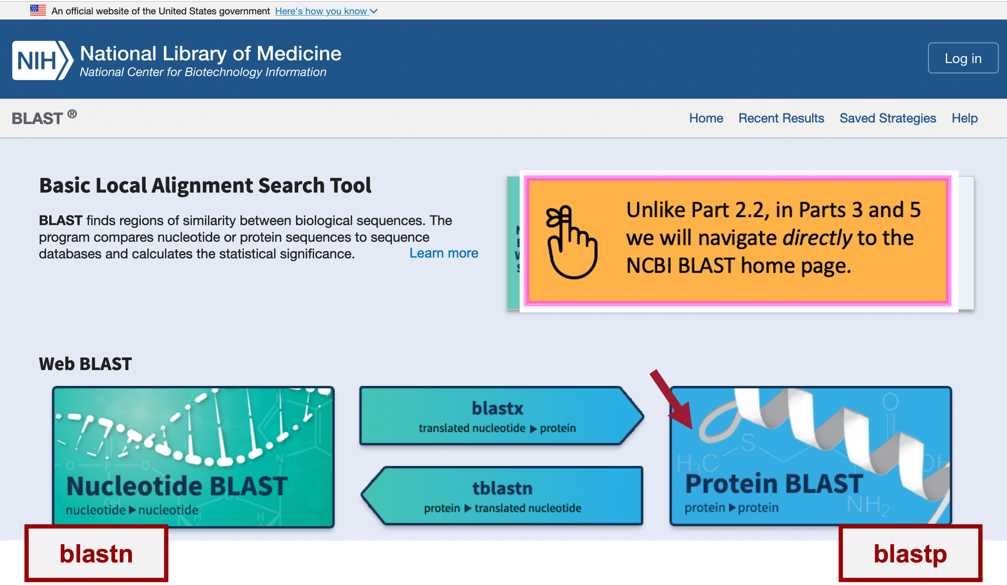
Navigate to NCBI BLAST.
-
Click on the “Protein BLAST” button (Figure 34).
-
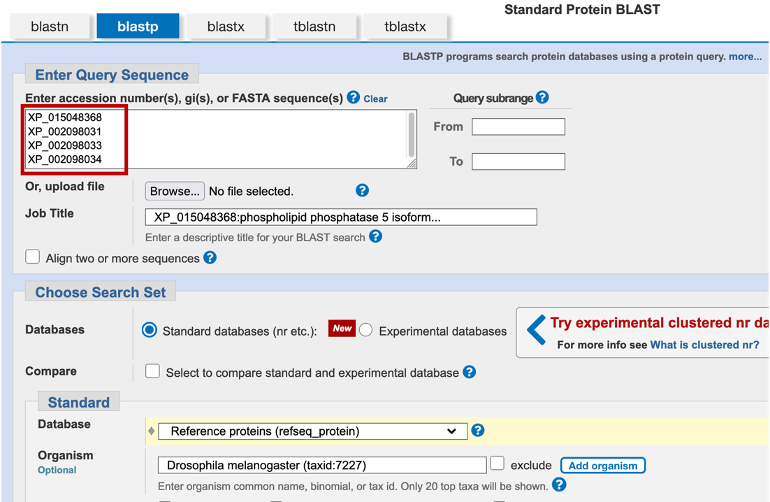
Paste the accession number for the translated protein sequence we copied from the GenBank Record for XM_039375862 (i.e., “XP_039231796”) into the “Enter Query Sequence” text box (Figure 35).
-
Under “Choose Search Set,” select “Reference proteins (refseq_protein)” in the drop-down menu under the “Database” field.
-
In the “Organism” text box, enter “Drosophila melanogaster (taxid:7227).”
-
Select the check box next to “Show results in a new window” then click on the “BLAST” button.
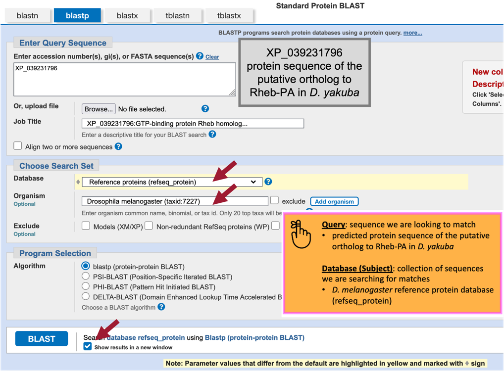
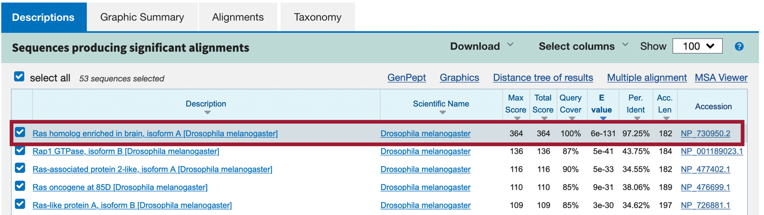
Our blastp search found 45 proteins within the D. melanogaster reference proteins (refseq_protein) database that show similarities with the protein sequence of the putative ortholog of Rheb-PA in D. yakuba (XP_039231796); however, only one of these is a good hit (Ras homolog enriched in brain, isoform A [Drosophila melanogaster]; accession: NP_730950, sequence identity of 97.25%, and an E-value of 6e-131). The remaining hits had much higher E-values (5e-41 to 0.002) and much lower percent identities (43.75% to 23.48%) (Figure 36). Therefore, the blastp search result shows that the D. yakuba RefSeq prediction XP_039231796 is most similar to the A isoform of Rheb among all the annotated proteins in D. melanogaster. Hence, based on parsimony, the blastp search result supports the hypothesis that XP_039231796 is the putative ortholog of Rheb in D. yakuba.
-
Now we need to repeat the blastp search (Steps 1-9 above) for the transcripts of the two neighboring genes on both sides of XM_039375862 (i.e., XM_002097995, XM_015192882, XM_002097997, and XM_002097998). See Figure 37 to help you stay oriented in the Genome Browser. See Appendix A for instructions on how to combine (or batch) multiple sequences.
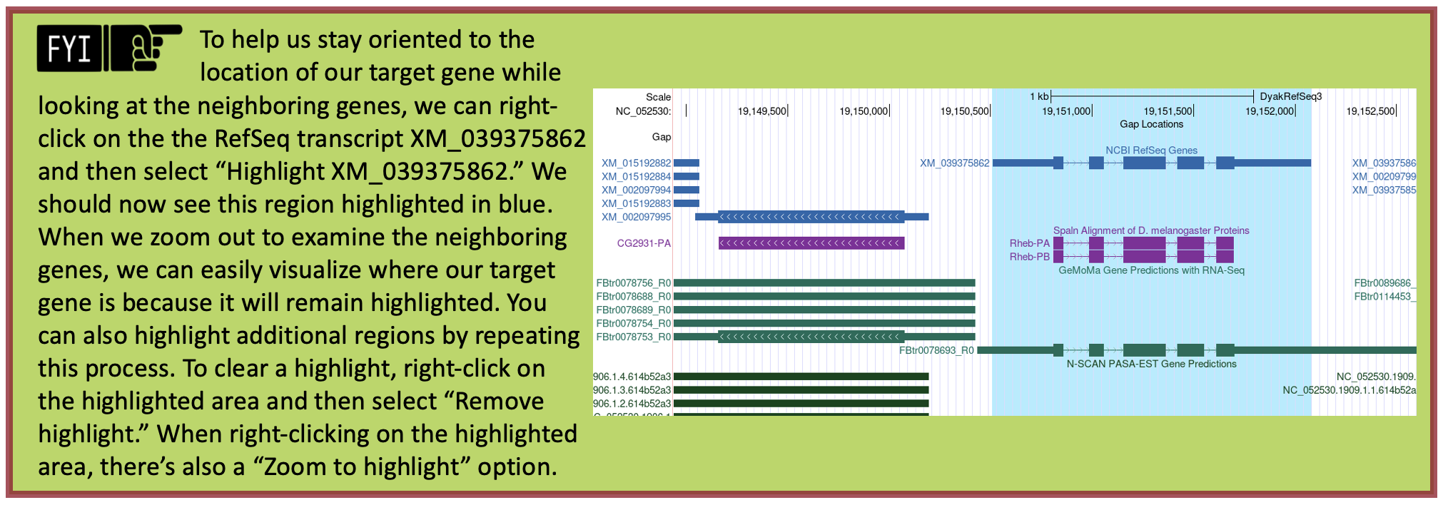
Now that we’ve examined the genomic neighborhood of the putative ortholog (Figure 39), we need to identify the direction of transcription for the putative ortholog of Rheb-PA and the neighboring genes in D. yakuba and then use this information to draw a sketch of the genomic neighborhood. To do so, we need to repeat the process we followed in Part 1 (i.e., zoom into an intron (or exon) of each gene and draw arrows in the correct directions on our sketch).
-
Use the strategy described in Steps 9 – 11 of Part 1 to determine the orientations of the putative Rheb ortholog (XM_039375862) and the transcripts of the two neighboring genes on both sides (i.e., XM_002097995, XM_015192882, XM_002097997 and XM_002097998) (Figure 40).
If the genomic neighborhood looks similar between Rheb in D. melanogaster (Figure 11) and the putative ortholog in D. yakuba (Figure 40), we can be confident we have found the best candidate for the ortholog. However, if any of the information is inconsistent with this being a locally syntenic region (local synteny: conservation of genomic neighborhood), we should inspect our other hits in the tblastn search (Part 2) to see if a different genomic region is a better match overall.
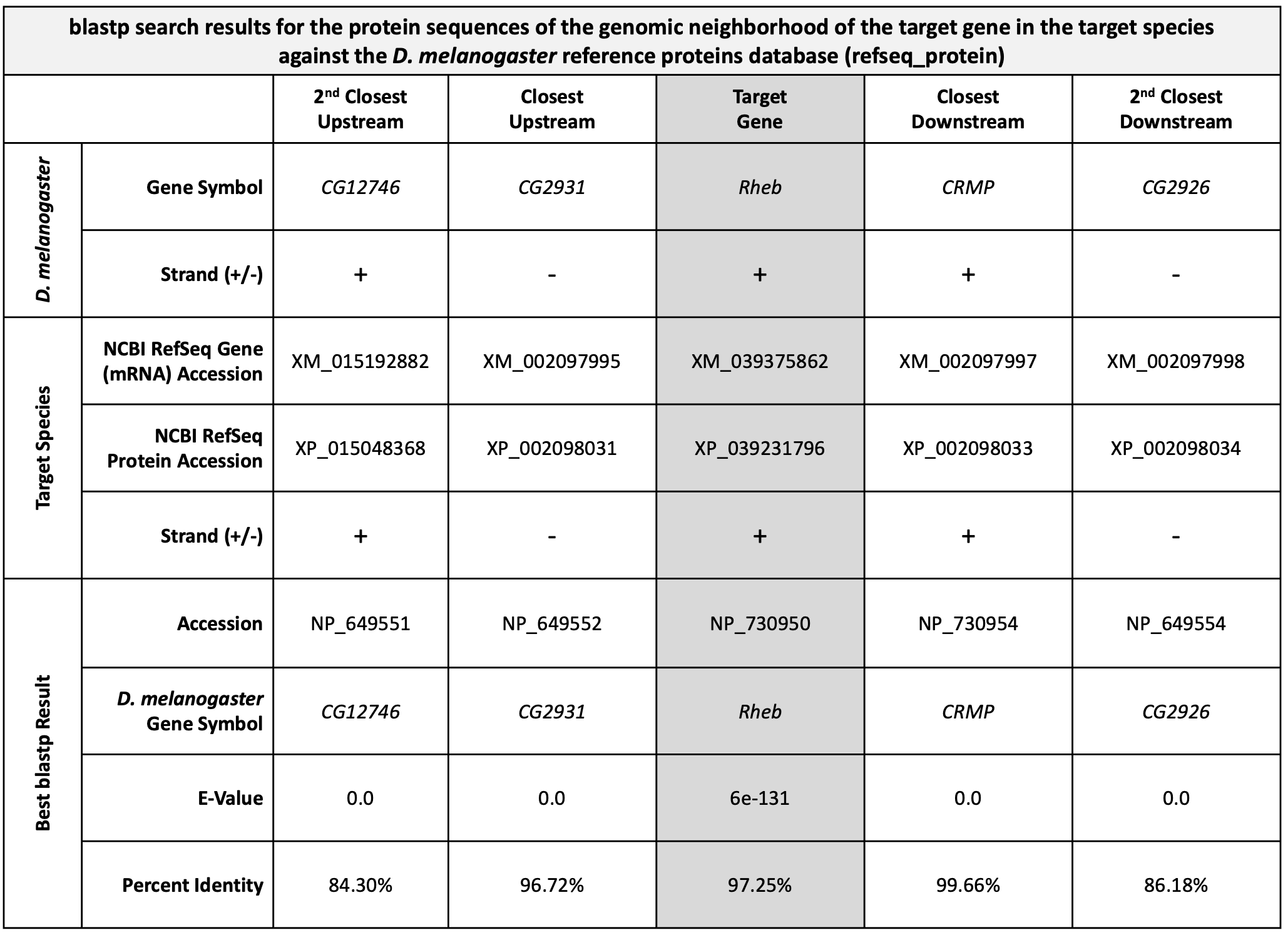
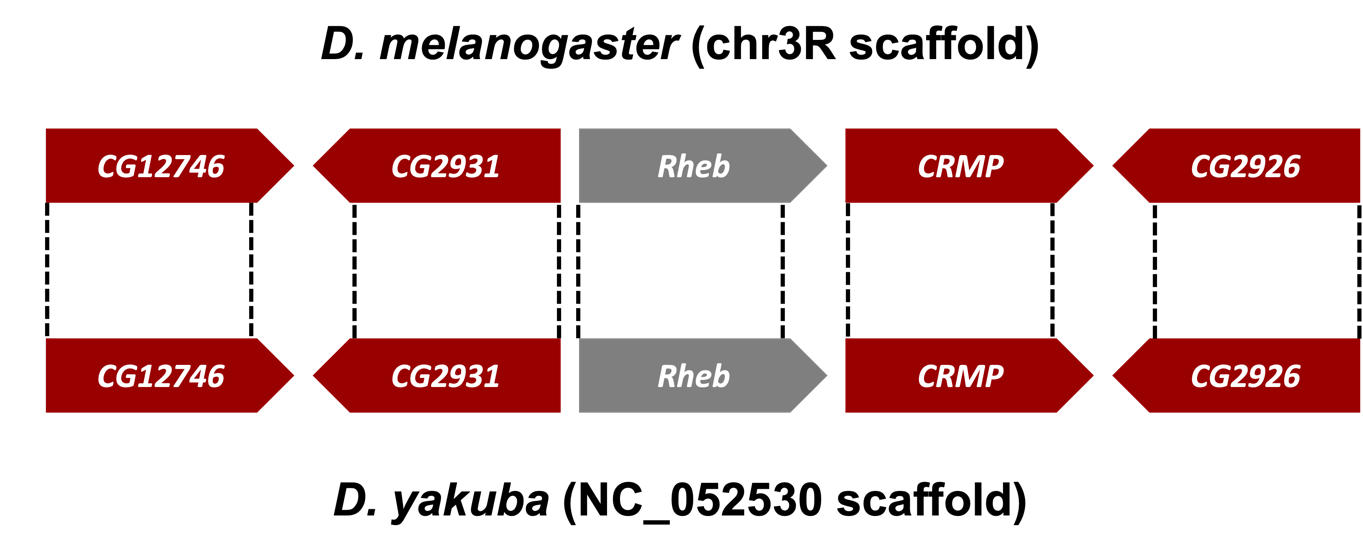
Examination of the genomic regions surrounding the Rheb gene in D. melanogaster (Figure 41; top) and the putative Rheb ortholog in D. yakuba (Figure 41; bottom) shows that the relative gene order (i.e., CG12746, CG2931, Rheb, CRMP, and CG2926) and orientations (+, -, +, + , -) are the same in the two species. Hence the synteny analysis supports the assignment of the D. yakuba feature at NC_052530:19,150,510-19,152,080 as an ortholog of Rheb.
|
|
If your target species' assembly happened to have been numbered from the opposite end of the relevant scaffold, the orientation (+ or – strand) of the orthologs could be the opposite (i.e., -, +, -, -, +) of what you see in D. melanogaster but still be syntenic. |
Part 4: Determine target gene’s structure in D. melanogaster
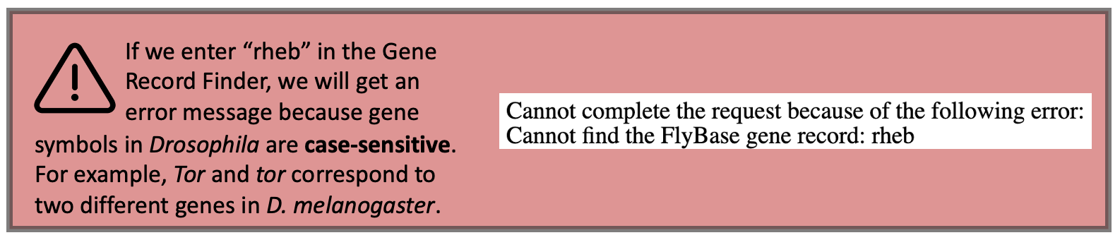
In Part 4 we will use the Gene Record Finder, which is a web tool that enables us to quickly identify the set of exons for a given gene and to retrieve their Coding DNA Sequences (CDS’s), also referred to as coding exons.
The Gene Record Finder will also provide details, such as number of isoforms, exon-intron structure and their coordinates, and transcript and protein information of the gene in question (in this case Rheb). It is important to remember that the details provided by the Gene Record Finder are for the gene in the reference species, D. melanogaster. We will use the details from Rheb in D. melanogaster to assist us with creating a gene model for Rheb in D. yakuba.
Before we can construct the orthologous gene model, we need to ascertain the gene structure (e.g., number of isoforms and CDS’s) of the D. melanogaster Rheb gene using the Gene Record Finder.
-
Open a new web browser tab and navigate to the Gene Record Finder.
-
Enter “Rheb” into the text box (Figure 42).
-
Click on the “Find Record” button (Figure 43).
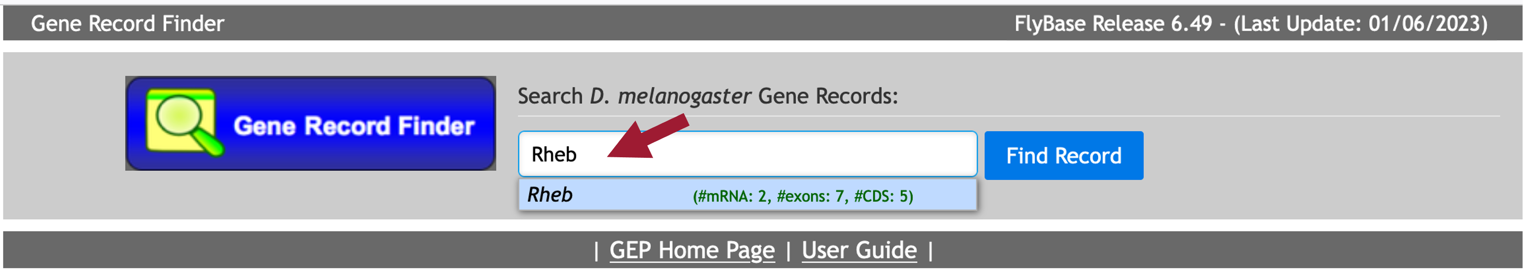
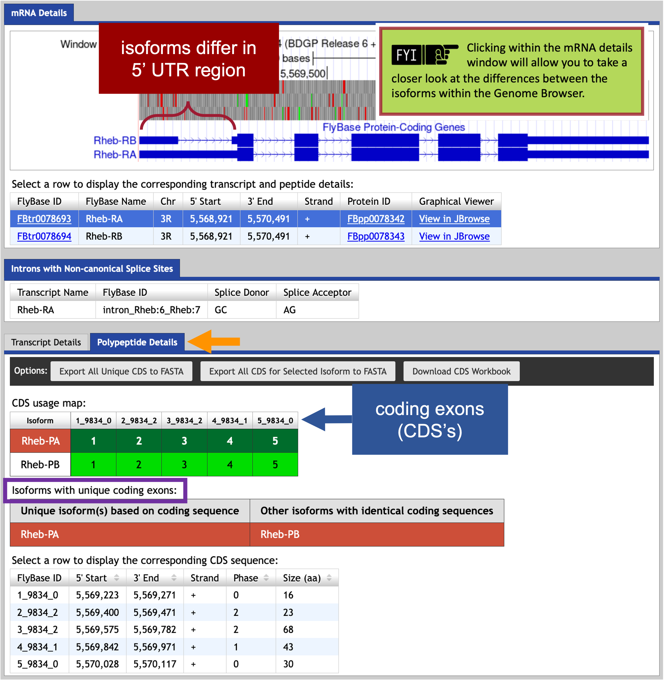
The Gene Record Finder shows that Rheb has two isoforms (A and B) in D. melanogaster. A graphical overview of the two isoforms is shown in the “mRNA Details” panel. The “CDS usage map” (under the “Polypeptide Details” tab) shows that both isoforms have the same set of coding exons (CDS’s) (i.e., 1_9812_0, 2_9812_2, 3_9812_2, 4_9812_1, and 5_9812_0). (The coding exons are ordered from 5' to 3' (from left to right) in the CDS usage map.) Hence the differences between these two isoforms are limited to the untranslated regions (UTRs) (Figure 45).

Part 5: Determine approximate location of coding exons (CDS’s) in target species
The initial tblastn search we performed in Part 2 helped define the search region for the putative ortholog within the genomic scaffold of the target genome, D. yakuba. The next step in our analysis is to determine the approximate coordinates of each coding exon (CDS) of Rheb-PA in D. yakuba. The approximate coordinates of each CDS can be determined by aligning each CDS of the gene in D. melanogaster against the search region (Figure 25) of the target genome (Figure 46).
In addition to comparing a query sequence against a collection of subject sequences in a database (e.g., Part 2 of this walkthrough), the NCBI BLAST web service also allows us to compare two or more sequences against each other (using the program bl2seq (BLAST 2 sequences)).
To map the amino acid sequences of each D. melanogaster CDS against the D. yakuba scaffold, BLAST must translate the entire D. yakuba scaffold sequence in all six reading frames (i.e., three reading frames of the positive strand and three reading frames of the negative strand) and then compare each conceptual translation against each CDS sequence from D. melanogaster. Thus, we will conduct a tblastn search using the CDS as the query and the nucleotide sequence of the scaffold as the subject.
Here, we will perform five tblastn searches — using each D. melanogaster Rheb CDS sequence as the query and the accession number (NC_052530) we identified for the D. yakuba scaffold in Part 2 (Figure 21) as the database (subject) sequence.
-
Scroll down to the CDS usage map (under the “Polypeptide Details” tab, Figure 47, orange arrow). Since Rheb has 5 CDS’s, we will need to run five different tblastn searches, one for each CDS. Let’s start with CDS-1 (Figure 47, red arrow).
-
To view the protein sequence for CDS-1, select row 1 (FlyBase ID: 1_9812_0).
-
Copy the protein sequence (including the header) shown in the pop-up window.

-
To setup the tblastn search, navigate to the NCBI BLAST website.
-
Click on the “tblastn” image under the “Web BLAST” section (Figure 48).
-
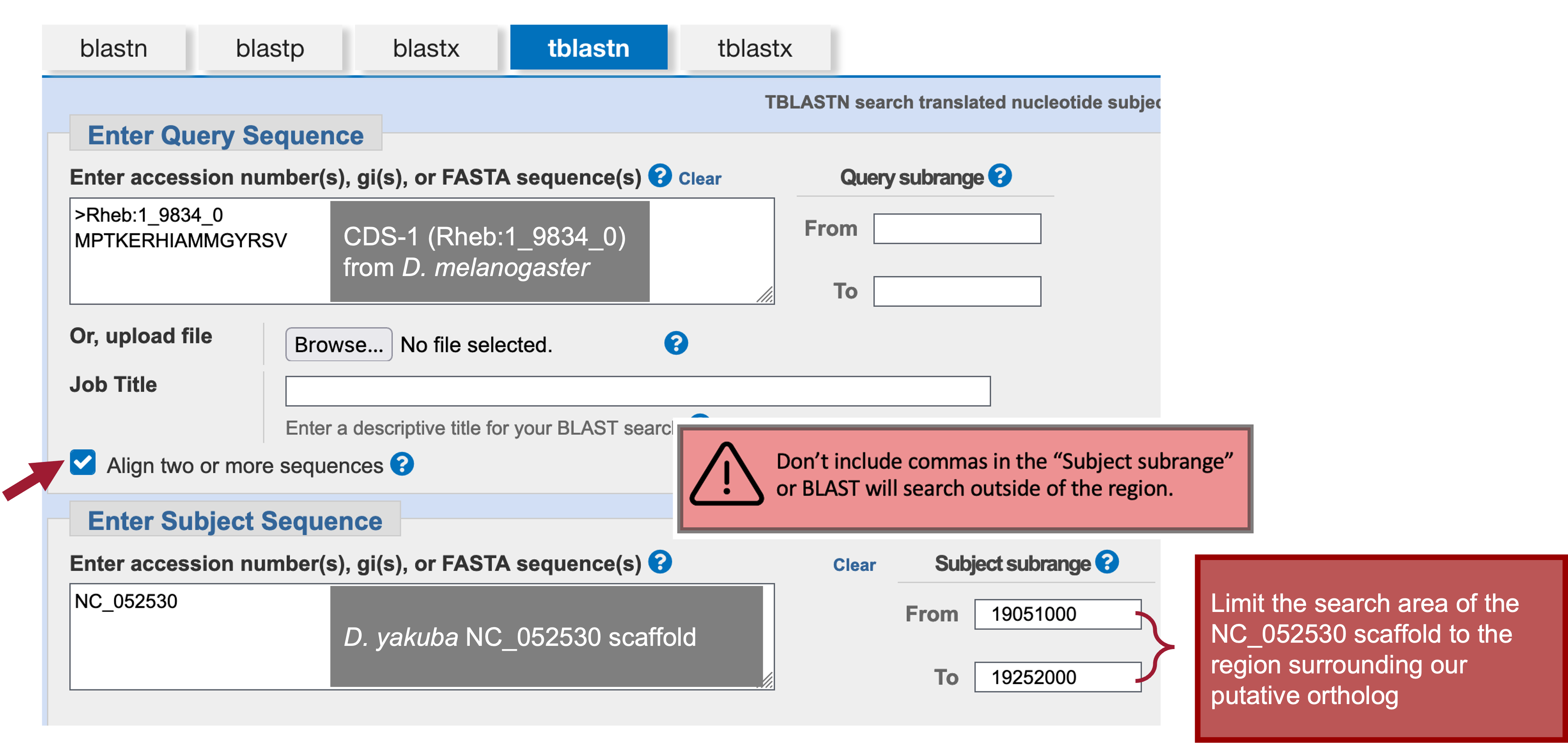
Paste the sequence for CDS-1 (i.e., 1_9812_0) into the “Enter Query Sequence” text box (Figure 49).
-
Select the “Align two or more sequences” checkbox.
NCBI BLAST is using the bl2seq (BLAST 2 sequences) program. -
In the “Enter Subject Sequence” text box, enter the Accession Number for the D. yakuba scaffold (i.e., “NC_052530”) we identified in Part 2.2.
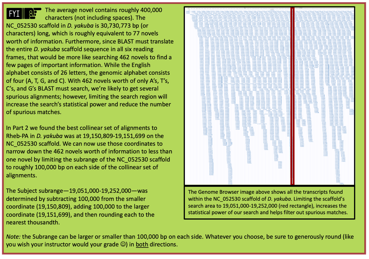
In Part 2 we found the best collinear set of alignments to Rheb-PA in D. yakuba was at 19,150,809-19,151,699 on the NC_052530 scaffold. We can now use those coordinates to narrow down the search region of the D. yakuba scaffold by limiting the subrange of the NC_052530 scaffold to roughly 100,000 bp on each side of the collinear set of alignments.
The Subject subrange—19,051,000-19,252,000—is determined by subtracting 100,000 from the smaller coordinate (19,150,809), adding 100,000 to the larger coordinate (19,151,699), and then rounding each to the nearest thousandth.
The default NCBI BLAST parameters are optimized for searching the query sequence against a large collection of sequences in a database. When we are using BLAST to compare only two sequences against each other, we need to change some of the algorithm parameters because the default parameters could potentially mask the conserved regions of the coding exon.
-
Click on the “+” icon next to “Algorithm parameters” to expand the section (Figure 51).
-
In the “Scoring Parameters” section, change the “Compositional adjustments” field to “No adjustment.”
-
In the “Filters and Masking” section, uncheck the “Low complexity regions” checkbox in the “Filter” field.
-
Select the check box next to “Show results in a new window” then click on the “BLAST” button.

The tblastn results (Figure 52, Figure 53) show a single match (E-value: 1e-06; sequence identity: 93.75%) to CDS-1 (Rheb:1_9812_0).
-
Click on the “Alignments” tab to view the corresponding tblastn alignment (Figure 54).
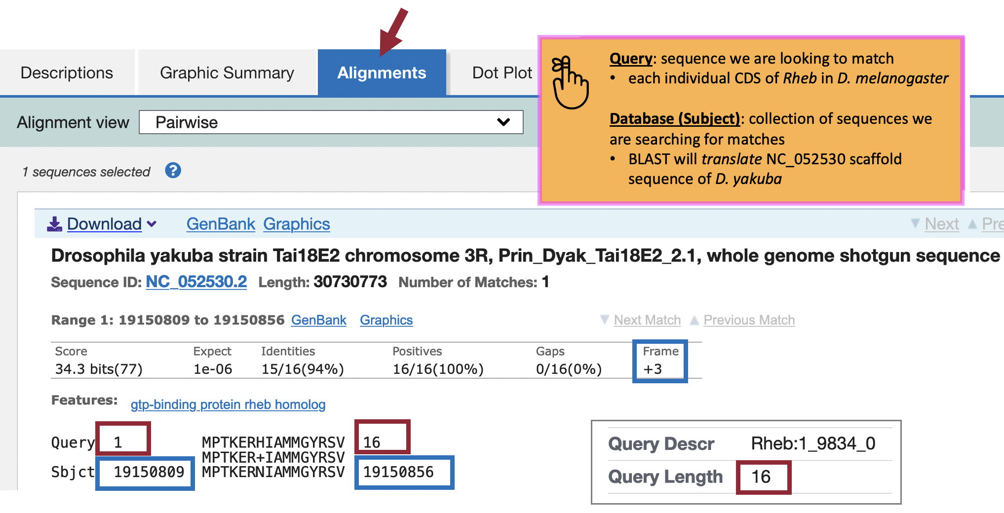
The “Query” coordinates show that the alignment covers all 16 amino acids (aa) of CDS-1 (Figure 54, red boxes).
|
|
We can find the length (in aa) of CDS-1 in D. melanogaster using the Gene Record Finder (“Size (aa)” column under the “Polypeptide Details” tab; Figure 47, circle) or at the top of the tblastn search results (Figure 52). |
The “Subject” coordinates correspond to the region within the NC_052530 scaffold of D. yakuba (i.e., 19,150,809 – 19,150,856) that shows sequence similarity to CDS-1 (Rheb:1_9812_0) from D. melanogaster when it is translated in the third reading frame of the positive strand (i.e., Frame +3). Hence, we can place CDS-1 of Rheb at approximately “NC_052530:19,150,809-19,150,856” in D. yakuba.
We can apply this same procedure to place the other four CDS’s on the NC_052530 scaffold of D. yakuba. See Appendix A for instructions on how to combine (or batch) multiple sequences.
-
Copy the CDS-2 (Rheb:2_9812_2) sequence (along with the header) from the Gene Record Finder.
-
Return to the tblastn web browser and delete the CDS-1 sequence from the “Enter Query Sequence” textbox.
-
Paste the CDS-2 sequence in the textbox (leave everything else the same as we had for CDS-1).
-
Click on the “BLAST” button to run the tblastn search.
-
Click on the “Alignments” tab to view the corresponding tblastn alignment.
-
Repeat Steps 15-19 to BLAST the remaining CDS’s (Figure 55).
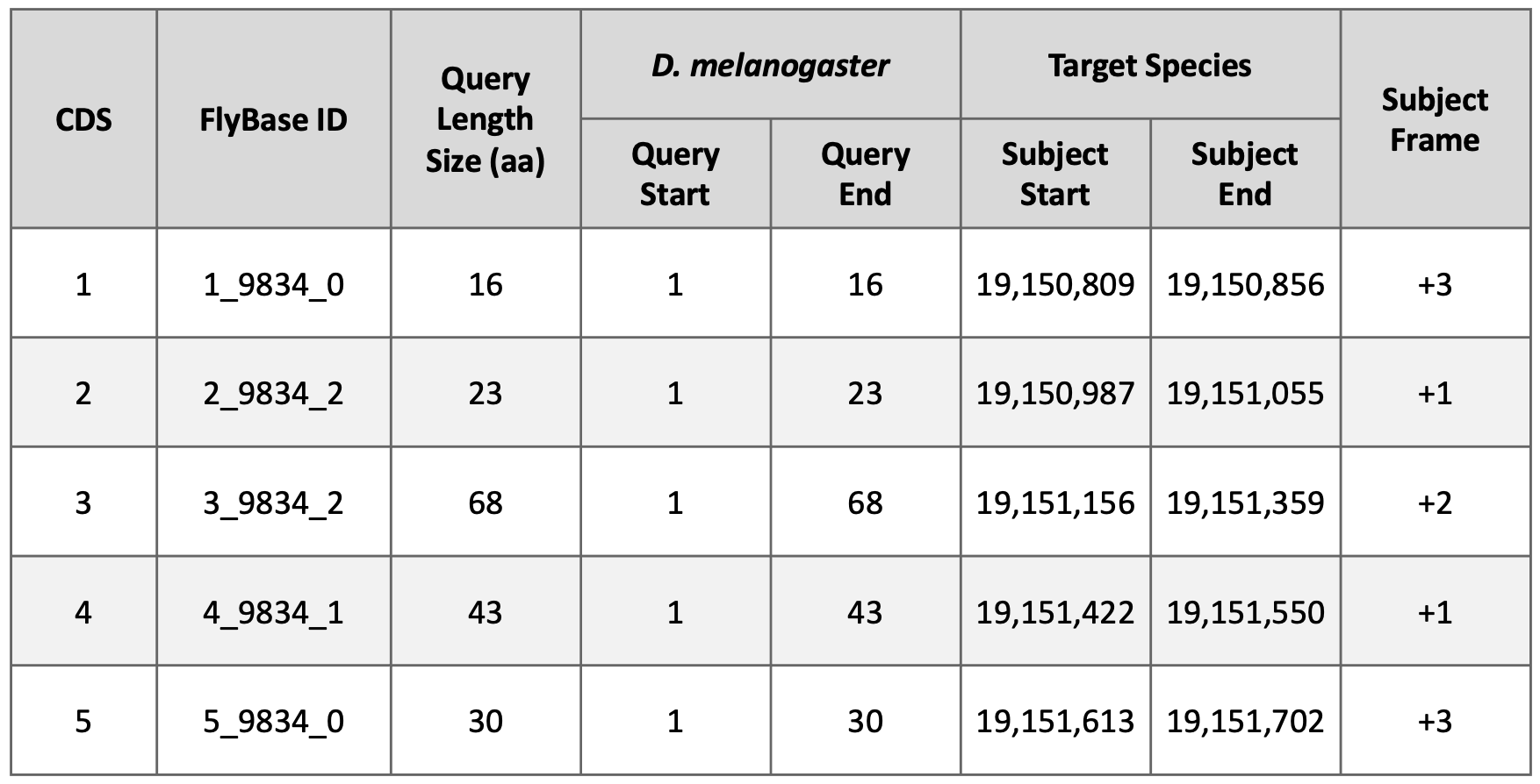
Examination of the subject ranges for the tblastn alignments of the five CDS’s of Rheb in D. yakuba shows that they are collinear—CDS’s 1-5 are placed on the positive strand and the subject ranges for the CDS’s are in ascending order. Consequently, the CDS-by-CDS search results support the hypothesis that the putative (probable) ortholog of Rheb-PA is located at approximately 19,150,809 – 19,151,702 on the NC_052530 scaffold of the D. yakuba genome assembly (i.e., NC_052530:19,150,809-19,151,702).
Part 6: Refine coordinates of coding exons (CDS’s)
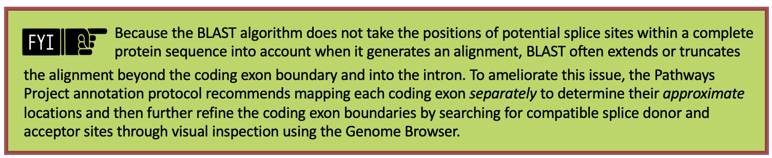
Now that we’ve mapped each CDS separately to determine their approximate locations (Figure 55), we will further refine the CDS boundaries by searching for compatible splice donor and splice acceptor sites by visual inspection using the Genome Browser (Figure 56).
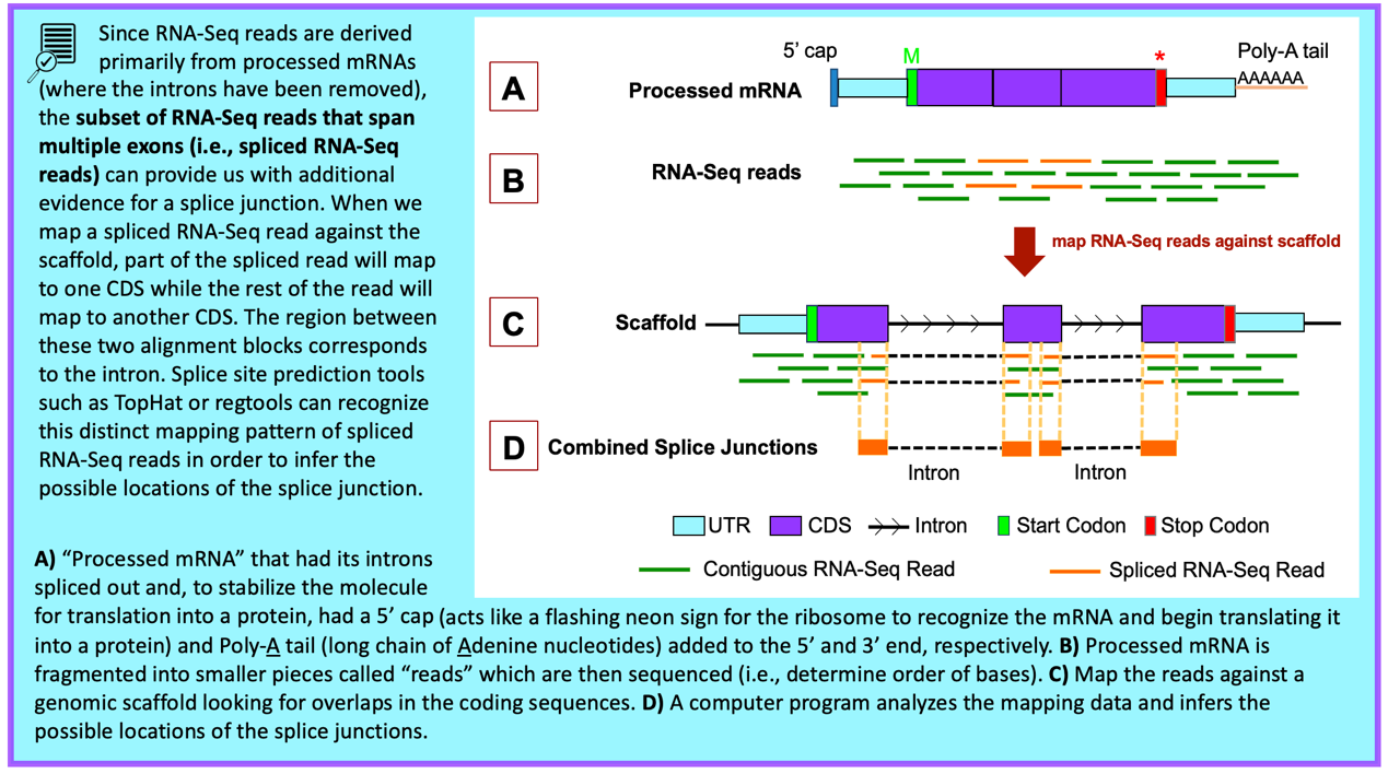
Previous studies by the modENCODE project and by other research projects (e.g., Yang et al., 2018) have generated RNA-Seq data for multiple tissues of D. yakuba at different developmental stages. These RNA-Seq reads (100–150 bp in length) are derived primarily from processed mRNA (i.e., after the introns have been removed). Hence, genomic regions with RNA-Seq read coverage usually correspond to transcribed exons, which include both the translated and untranslated regions.
The “Aggregated RNA-Seq Coverage” evidence track shows the sum of the RNA-Seq coverage from all the samples available on the Genome Browser for the target species (Figure 57). The height of the histogram correlates with the total number of RNA-Seq reads that have been mapped to each position of the D. yakuba scaffold. By default, the scale of the “Aggregated RNA-Seq Coverage” track will change automatically based on the minimum and maximum read depth within the genomic region being viewed.
RNA-Seq read coverage for specific developmental stages and tissues are available under the “RNA-Seq Tracks” section of the Genome Browser. For D. yakuba, RNA-Seq read coverage for adult females and adult males are available through the “RNA-Seq Coverage (Stages)” composite track. RNA-Seq read coverage for seven tissues (i.e., head, thorax, abdomen, digestive system, gonad, reproductive tract, and whole body) in females and males are available under the “RNA-Seq Coverage (Tissues)” composite track.
Part 6.1: Verify start codon coordinates
We need to ascertain whether the tblastn alignment for CDS-1 at 19,150,809-19,150,856 (Figure 57) is supported by RNA-Seq data and, if so, determine the location of the start codon.
-
Return to the Genome Browser for D. yakuba.
-
To examine the region of the tblastn alignment for CDS-1, enter “NC_052530:19,150,809-19,150,856” into the “enter position or search terms” text box.
-
Under the “Mapping and Sequencing Tracks,” change the “Base Position” track to “full.”
-
Click on any “refresh” button.
The “Aggregated RNA-Seq Coverage” track show high RNA-Seq read depth within the tblastn alignment block (19,150,809-19,150,856), consistent with the hypothesis that this region is being transcribed in D. yakuba.
Notice that Frame +1 of this region has two stop codons (denoted in red with an “*”) while Frames +2 and +3 have an Open Reading Frame (i.e., no stop codons are shown within Frames +2 or +3 of CDS-1).
-
To examine the region surrounding the start of the tblastn alignment to CDS-1, enter “NC_052530:19,150,809” into the “chromosome range or search terms” text box.
-
Click on the “go” button.
-
Zoom out 3x and another 10x.
In Part 5 (Figure 54), we found our tblastn alignment for CDS-1 begins at approximately 19,150,809 (Figure 57, highlighted blue). Examination of this region using the Genome Browser shows us that Frame +3 has a start codon in this location and is supported by multiple evidence tracks—the NCBI RefSeq Genes and Spaln alignment of D. melanogaster proteins, and gene predictors GeMoMa, N-SCAN, and Augustus (Figure 57).
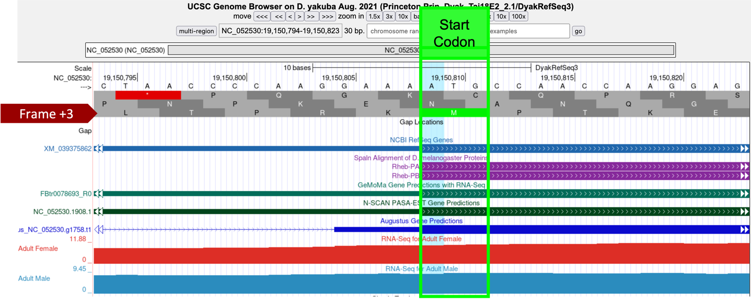
The tblastn alignment for CDS-1 (CDS 1_9812_0) of Rheb in D. melanogaster against the D. yakuba scaffold encompasses all 16 amino acids of the CDS (Figure 54), and the alignment begins with a start codon at 19,150,809-19,150,811. Hence the most parsimonious gene model for Rheb-PA in D. yakuba would use the start codon at 19,150,809-19,150,811 in scaffold NC_052530.
Part 6.2: Verify stop codon coordinates
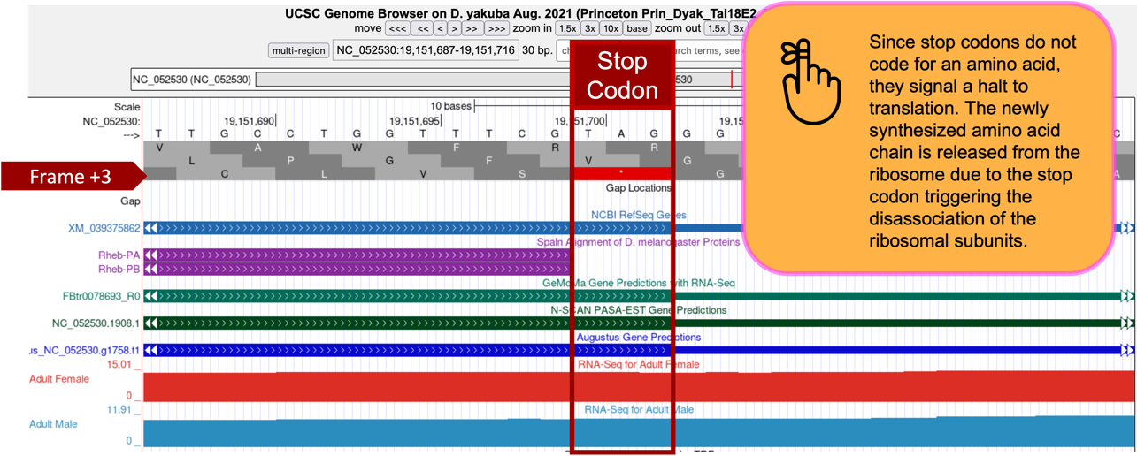
In Part 5 (Figure 55), we found our tblastn alignment for CDS-5 ends at approximately 19,151,702 when translated in Frame +3. The alignment covers all 30 amino acids of CDS-5 and ends with a stop codon (Figure 58).

-
To examine the genomic region surrounding the end of the tblastn alignment to CDS-5, enter “NC_052530:19,151,702” into the “chromosome range or search terms” text box.
-
Click on the “go” button.
-
Zoom out 3x and another 10x (Figure 59).
The stop codon at 19,151,700-19,151,702 is consistent with the NCBI RefSeq Genes and Spaln alignment of D. melanogaster proteins (stop codons don’t become part of the protein rather they signal when translation should terminate and the newly made protein should be released), and gene predictors GeMoMa, N-SCAN, and Augustus.
Based on the tblastn alignment for CDS-5 and the available evidence on the Genome Browser, the stop codon for the Rheb-PA ortholog is placed at 19,151,700-19,151,702, and the last codon (S; Serine), before the stop codon, ends at 19,151,699 (Figure 59).
Note that the “Aggregated RNA-Seq Coverage” track indicates that transcription extends beyond the stop codon. Based on the gene structure of Rheb-RA in D. melanogaster, the region with RNA-Seq read coverage that extends beyond the stop codon likely corresponds to the 3' untranslated region (UTR) of the last exon in Rheb.
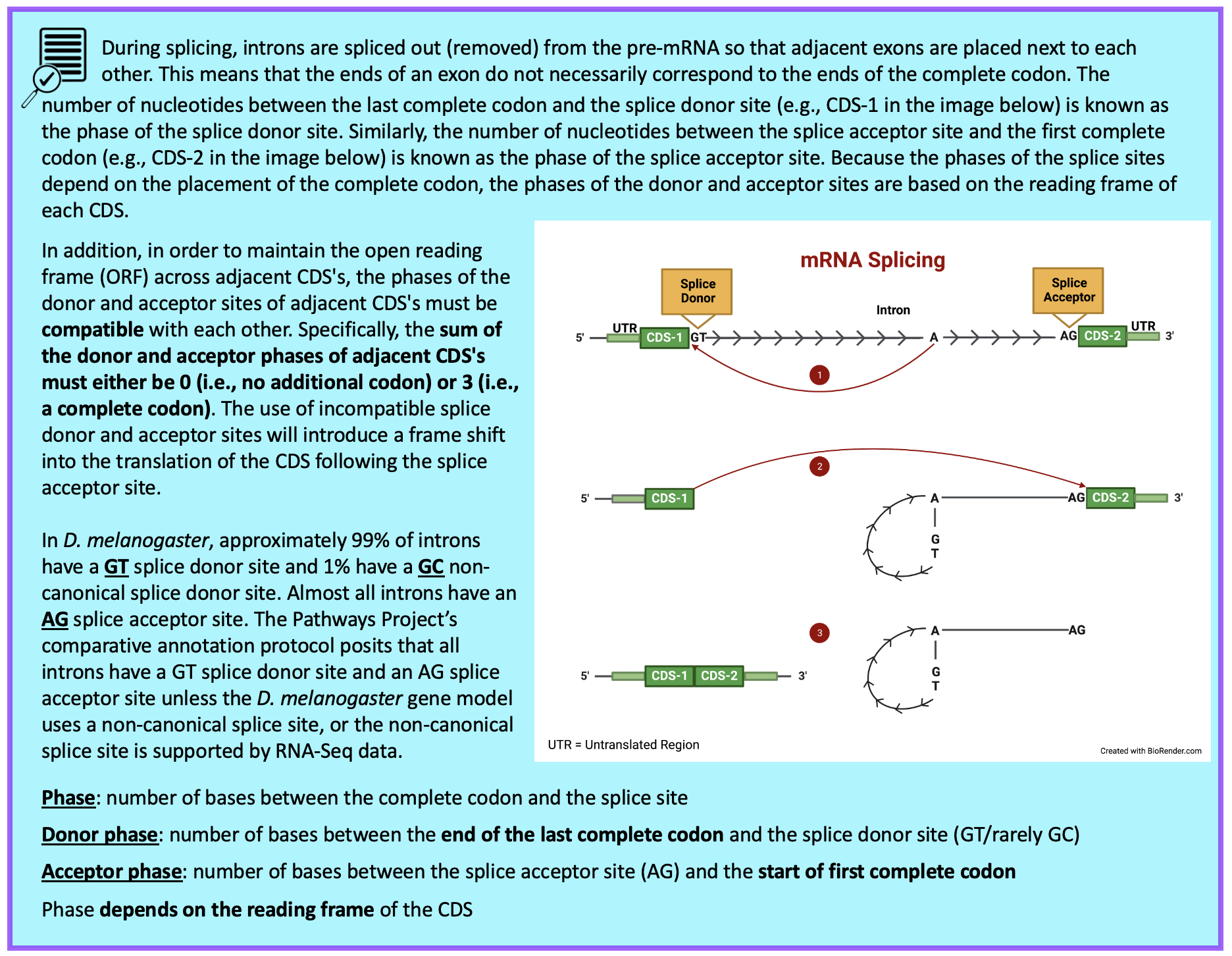
Part 6.3: Determine phases of donor and acceptor splice sites
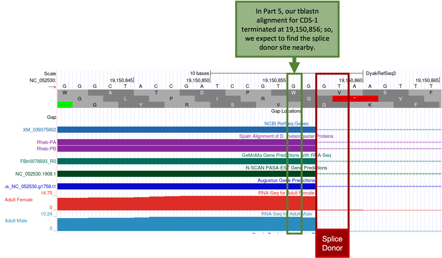
Because the tblastn alignment for CDS-1 of Rheb terminates at 19,150,856 (Figure 54), we expect to find the splice donor site for CDS-1 at around position 19,150,856.
-
To examine the genomic region surrounding the splice donor site of CDS-1, enter “NC_052530:19,150,856” into the “chromosome range or search terms” text box.
-
Click on the “go” button.
-
Zoom out 3x and another 10x to examine the 30 bp surrounding this position.
The GT splice donor site closest to 19,150,856 (Figure 61, green box) is located at 19,150,858-19,150,859 (Figure 61, red box) which is supported by multiple lines of evidence—NCBI RefSeq Genes, Spaln alignment of D. melanogaster proteins, and the GeMoMa, N-SCAN, and Augustus gene predictions, and the aggregated RNA-Seq read coverage.
-
Zoom out far enough to see the entire length of CDS-1 and confirm that Frame +3 has an Open Reading Frame (ORF) (i.e., no stop codons are shown within Frame +3 of CDS-1).
Using tblastn in Part 5, we determined the approximate location of CDS-1 was 19,150,809-19,150,856. Using the Genome Browser, in Part 6.1 we verified the start codon of CDS-1 was in Frame +3 at 19,150,809-19,150,811 (Figure 57). We visually inspected the region surrounding the approximate end of CDS-1 and placed the splice donor site at 19,150,858-19,150,859, after which we confirmed Frame +3 of CDS-1 has an ORF. Now we need to determine the phase of the splice donor site for CDS-1.
-
Enter “NC_052530:19,150,849-19,150,859” into the “chromosome range or search terms” text box and click on “go.”
In Figure 62, we see the last complete codon (i.e., containing three nucleotides) of CDS-1 before the splice donor site codes for the amino acid Tryptophan in Frame +1, Arginine in Frame +2, and Valine in Frame +3.
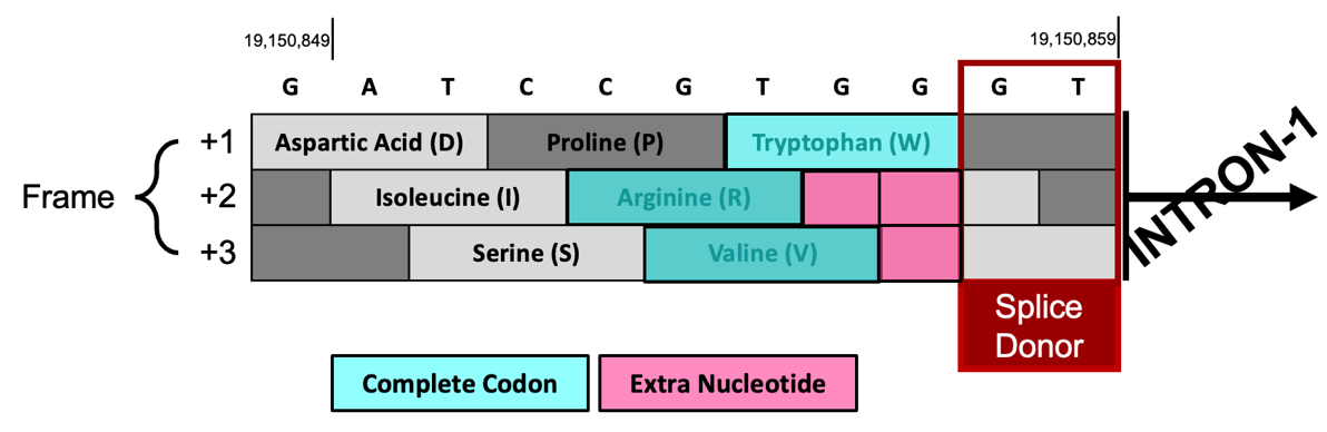
The splice donor site at 19,150,858-19,150,859 is in phase 0 relative to Frame +1 because CDS-1 ends in a complete codon and thus has no extra nucleotides. In contrast, Frame +2 and Frame +3 don’t end in complete codons so they each have extra nucleotides. The splice donor site is in phase 2 relative to Frame +2 because there are 2 extra nucleotides (GG) after the last complete codon. The splice donor site is in phase 1 relative to Frame +3 since there is 1 extra nucleotide (G) after the last complete codon (Figure 62).
We previously determined CDS-1 is translated in Frame +3 (Figure 57); therefore, the last complete codon of CDS-1 (GTG which codes for Valine (V)) is located at 19,150,854-19,150,856 and there is one extra nucleotide (G at 19,150,857) between the last complete codon and the splice donor site. Hence, the CDS-1 splice donor site is in phase 1.
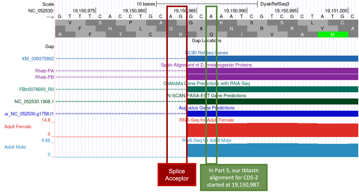
Our tblastn alignment in Part 5 placed CDS-2 at approximately 19,150,987 – 19,151,055 (Figure 55); therefore, we expect to find the splice acceptor site for CDS-2 around position 19,150,987.
-
To examine the genomic region surrounding the splice acceptor site of CDS-2, enter “NC_052530:19,150,987” into the “chromosome range or search terms” text box and click on “go.”
-
Zoom out 3x and another 10x to examine the 30 bp surrounding this position (Figure 63).
There is only one potential canonical (“standard rule”) splice acceptor site (AG) in the 30 bp region surrounding the start of the tblastn alignment to CDS-2 (Figure 63, green box). The splice acceptor site is located at 19,150,983-19,150,984 (Figure 63, red box) and is supported by the NCBI RefSeq Genes and Spaln alignment of D. melanogaster proteins, the GeMoMa, N-SCAN, and Augustus gene predictions, and the aggregated RNA-Seq read coverage. Thus, CDS-2 starts at 19,150,985.
Now we need to determine the frame in which CDS-2 is translated.
-
Enter “NC_052530:19,150,980-19,150,990” into the “search terms” text box and click on “go” to zoom in on the region surrounding the splice acceptor site.
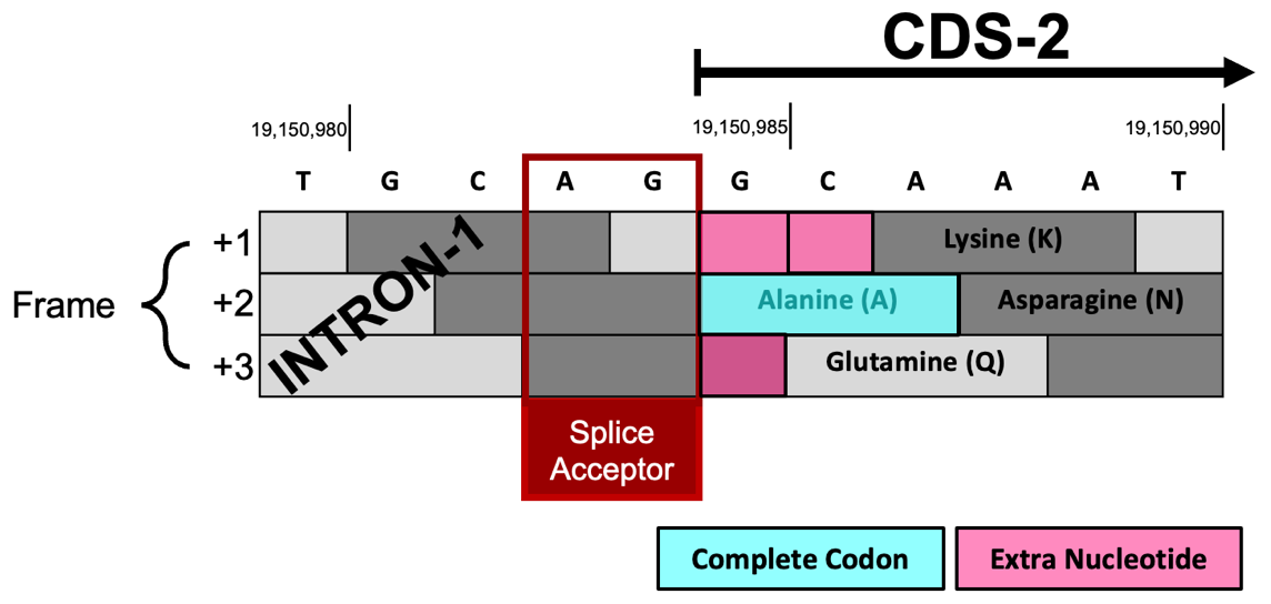
Each frame can have extra nucleotides (0, 1, or 2) between the beginning of CDS-2 at 19,150,985 and the first complete codon of each frame (Figure 64).
-
Frame +1 has two extra nucleotides (GC) before the first complete codon (Lysine; K).
-
Splice acceptor site is in phase 2 relative to Frame +1.
-
-
Frame +2 begins with a complete codon (Alanine; A) so it has zero extra nucleotides.
-
Splice acceptor site is in phase 0 relative to Frame +2.
-
-
Frame +3 has one extra nucleotide (G) before the first complete codon (Glutamine; Q).
-
Splice acceptor site is in phase 1 relative to Frame +3.
-
Since the CDS-1 splice donor site at 19,150,858 – 19,150,859 is in phase 1 relative to Frame +3 (i.e., CDS-1 ends with one extra nucleotide), the CDS-2 splice acceptor site must be in phase 2 (i.e., CDS-2 must begin with two extra nucleotides) to maintain the ORF after Intron-1 has been removed. Since CDS-1 had one extra nucleotide (G) between the last complete codon (GTG = Valine; V) and the splice donor site, CDS-2 must start with two extra nucleotides to join the extra one from CDS-1 because we need 3 nucleotides to make a complete codon.
Since CDS-2 is in Frame +1 and the first complete codon (AAA codes for K) is located at 19,150,987- 19,150,989, there are two nucleotides (GC at 19,150,985- 19,150,986) between the potential splice acceptor site and the first complete codon. Hence, the CDS-2 splice acceptor site is in phase 2.
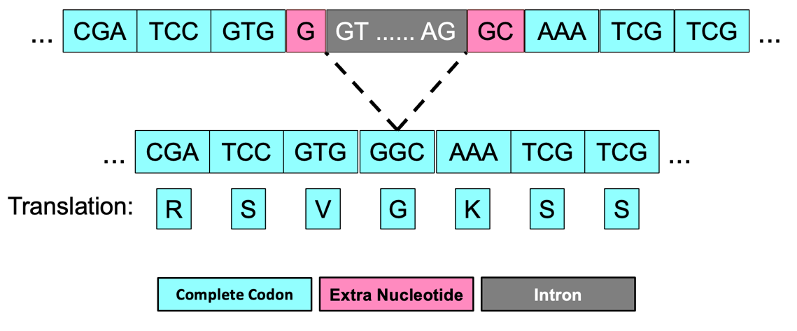
The extra nucleotides near the splice sites (i.e., G + GC) will form an additional amino acid (Glycine/G) after splicing (Figure 65). Collectively, our analysis suggests that CDS-1 ends at 19,150,857 with a phase 1 splice donor site and CDS-2 begins at 19,150,985 with a phase 2 splice acceptor site.
The same annotation strategy can be used to determine the phases for the remaining splice donor and splice acceptor sites between CDS-2 and CDS-3, CDS-3 and CDS-4, and CDS-4 and CDS-5 (Figure 66).
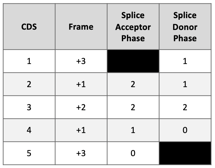
We reviewed the phases of splice donor and acceptor sites in Figure 60. Recall that to maintain the open reading frame (ORF) across adjacent CDS’s, the phases of the donor and acceptor sites of adjacent CDS’s must be compatible with each other (i.e., the sum of the donor and acceptor phases of adjacent CDS’s must either be 0 or 3).
Looking at the splice sites between CDS-1 and CDS-2, we see the splice donor phase of CDS-1 is one and the splice acceptor phase of CDS-2 is two. Thus, the sum of the donor and acceptor phases for Intron-1 is three (Figure 67).

Part 6.4: Use spliced RNA-Seq reads to verify coordinates for Intron-1
-
Under the “RNA Seq Tracks,” change the “Combined Splice Junctions” track to “pack.”
The “Combined Splice Junctions” track shows splice junctions extracted from spliced RNA-Seq reads that have been aligned to the genome. -
Click on the “refresh” button.
-
To examine the region surrounding Intron-1 (i.e., intron between CDS-1 and CDS-2), enter “NC_052530:19,150,858-19,150,984” into the “search terms” text box.
We found these coordinates in Part 6.3. Since our analysis in Part 6.3 suggested that CDS-1 ends at 19,150,857, Intron-1 should begin at 19,150,858; furthermore, we found that CDS-2 begins at 19,150,985 thus Intron-1 should end at 19,150,984. -
Click on the “go” button then zoom out 3x to examine the 381 bp surrounding this position (Figure 69).

There is only one splice junction predicted in this region.
-
To examine the splice donor site predicted by the splice junction JUNC00113127, zoom into the region surrounding the beginning of the intron predicted by this junction (Figure 69, purple arrow).
-
To examine the splice acceptor site predicted by the splice junction JUNC00113127, zoom into the region surrounding the end of the intron predicted by this junction (Figure 69, orange arrow).
The splice junction between the phase 1 donor site of CDS-1 and the phase 2 acceptor site of CDS-2 is supported by the NCBI RefSeq Genes and Spaln alignment of D. melanogaster proteins, gene predictors GeMoMa, N-SCAN, and Augustus, and the RNA-Seq data.
The score tells us how many spliced RNA-Seq reads there are that support a predicted splice junction. Since JUNC00113127 has a score of 6257, that splice junction prediction is supported by 6,257 spliced RNA-Seq reads. Splice junction predictions are color-coded based on the number of spliced RNA-Seq reads that support the junction (i.e., their scores). Based on the color-coded table in the “Description” section, JUNC00113127 will be red in the Genome Browser image since greater than 1,000 spliced RNA-Seq reads support the feature (Figure 70, bottom).

Based on multiple lines of evidence, we can conclude the splice junction prediction JUNC00113127 is consistent with our splice donor site for CDS-1 at 19,150,858-19,150,859 and our splice acceptor site for CDS-2 at 19,150,983-19,150,984 that we annotated in Part 6.3.
Part 6.5: Use splice junction predictions to verify coordinates for second intron
The same annotation strategy can be used to determine the coordinates for Intron-2 between CDS-2 and CDS-3.
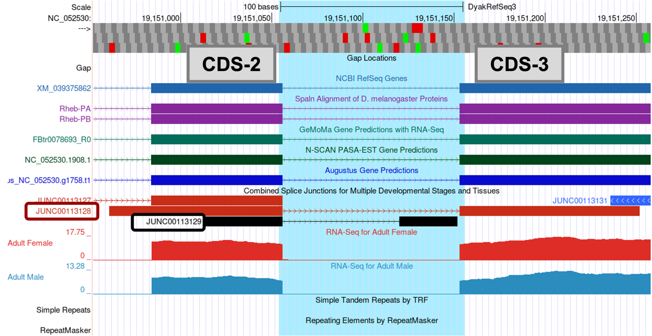
There are two splice junctions predicted in this region, JUNC00113128 and JUNC00113129.
The tblastn alignment for CDS-2 ends at 19,151,055 (Figure 55). The potential splice donor site at 19,151,057-19,151,058 for CDS-2 is supported by the splice junction predictions JUNC00113128 and JUNC00113129, the NCBI RefSeq Genes and Spaln alignment of D. melanogaster proteins, gene predictors GeMoMa, N-SCAN, and Augustus, and the RNA-Seq data. There is one nucleotide (A at 19,151,056) between the last complete codon (AAC) and the potential splice donor site. Hence, this splice donor site is in phase 1 relative to Frame +1.
The tblastn alignment for CDS-3 spans from 19,151,156-19,151,359 in Frame +2 (Figure 55). The potential splice acceptor site at 19,151,152-19,151,153 for CDS-3 is supported by the splice junction prediction JUNC00113128, the NCBI RefSeq Genes and Spaln alignment of D. melanogaster proteins, gene predictors GeMoMa, N-SCAN, and Augustus, and the RNA-Seq data. There are two nucleotides (CC at 19,151,154-19,151,155) between the first complete codon (TTC) and the potential splice acceptor site. Hence, this splice acceptor site is in phase 2 relative to Frame +2. This phase 2 splice acceptor site is compatible with the phase 1 splice donor site for CDS-2.
-
Click on the “JUNC00113128” feature to determine the number of spliced RNA-Seq reads that support this splice junction prediction (Figure 72).
-
Click on the back button of the web browser to return to the Genome Browser image.

In addition to the splice junction JUNC00113128, which supports the proposed splice acceptor site for CDS-3 at 19,151,152-19,151,153, there is another splice junction which suggests a different splice acceptor site (JUNC00113129) (Figure 71).
Thus, we need to investigate whether predicted junction JUNC00113129 is supported by other lines of evidence. CDS-3 in D. yakuba includes two methionine in Frame +2 (at 19,151,255-19,151,257 and 19,151,348-19,151,350). Hence, the splice junction JUNC00113129 could indicate the presence of a novel isoform of Rheb in D. yakuba. However, when we assess the number of spliced RNA-Seq reads that support the splice junction JUNC00113129, we find that this junction is weakly supported by only 8 spliced RNA-Seq reads; thus, there is little evidence to postulate a novel isoform of Rheb in D. yakuba based on this splice junction prediction.
|
|
In addition to the scores, when analyzing multiple splice junction predictions for an intron, be sure to confirm the predictions are on the same strand as the gene you’re annotating. For example, if a splice junction is predicted in the negative strand and the Rheb gene is on the positive strand relative to the D. yakuba NC_052530 scaffold, you could eliminate that prediction. |
Taking into account the splice site phases we found in Part 6.3 (Figure 66) and using Parts 6.4 and 6.5 as a guide, you will be able to find the start and end coordinates of the remaining CDSs for the gene model of Rheb-PA in D. yakuba (Figure 73).
Part 7: Verify and submit gene model(s)
Now that we’ve completed the annotation of Rheb-PA in D. yakuba, we need to verify our proposed gene model and prepare the corresponding sequence files for submission.
Part 7.1: Verify gene model of protein
Our analysis of the CDS-by-CDS tblastn alignments and the evidence tracks on the Genome Browser allowed us to precisely define the start and end positions of each of the five coding exons (CDS’s) of Rheb-PA. To verify that our proposed gene model satisfies the basic biological constraints (e.g., begins with a start codon, has compatible splice sites, and ends with a stop codon), we will check our gene model coordinates using the Gene Model Checker.
-
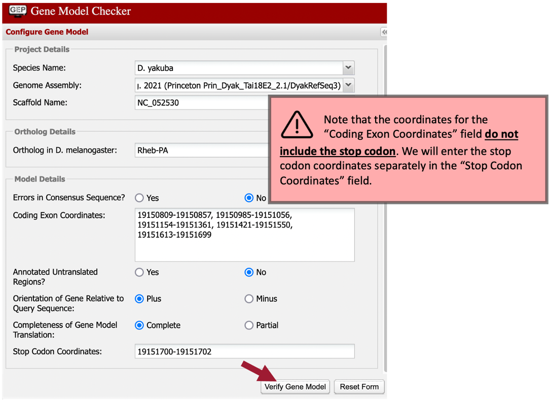
Open a new web browser tab and navigate to the Gene Model Checker (Figure 74).
-
In the “Project Details” section:
-
Species Name: select “D. yakuba”
-
Genome Assembly: select “Aug. 2021 (Princeton Prin_Dyak_Tai18E2_2.1/DyakRefSeq3)”
-
Scaffold Name: enter “NC_052530”
-
-
In the “Ortholog Details” section:
-
Ortholog in D. melanogaster: enter “Rheb-PA”
-
-
In the “Model Details” section:
-
Errors in Consensus Sequence? select “No”
-
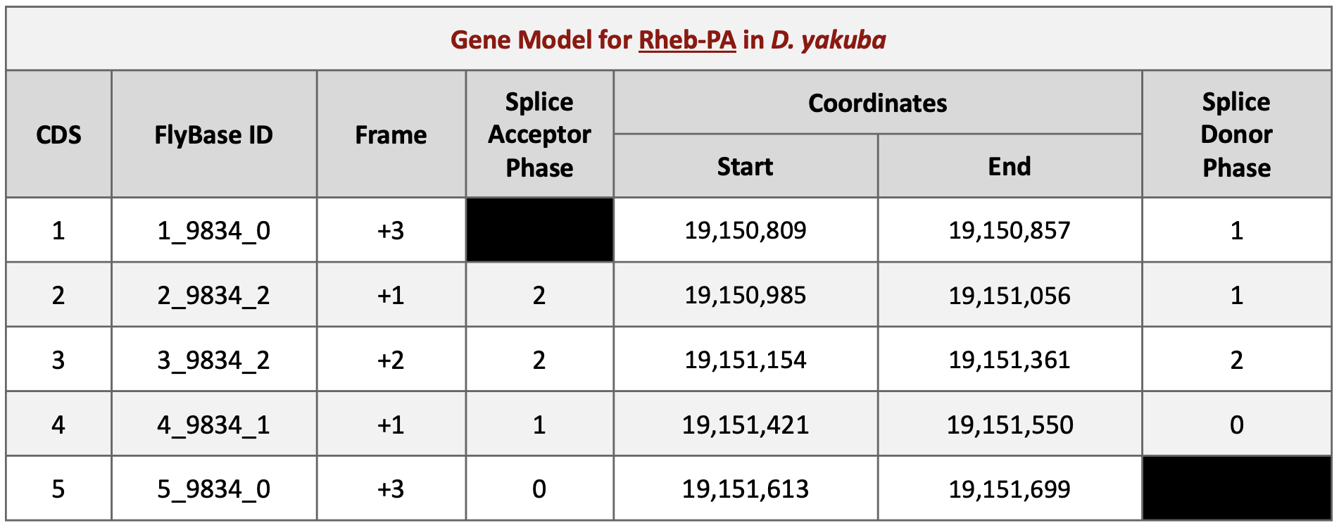
Coding Exon Coordinates: enter a comma-delimited list of coordinates for the five CDS’s as shown below (commas separate adjacent CDS’s; NO commas are included within each set of coordinates):
-
19150809-19150857, 19150985-19151056, 19151154-19151361, 19151421-19151550, 19151613-19151699
-
-
Annotated Untranslated Regions? select “No”
-
Orientation of Gene Relative to Query Sequence: select “Plus” since Rheb-PA is on the positive strand relative to the scaffold
-
Completeness of Gene Model Translation: select “Complete”
-
Stop Codon Coordinates: click within the textbox and the coordinates will automatically populate
-
-
Click on the “Verify Gene Model” button to run the Gene Model Checker.
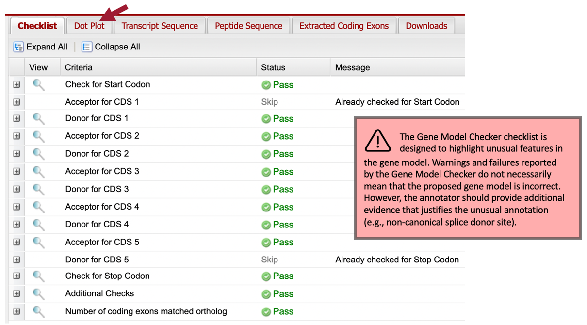
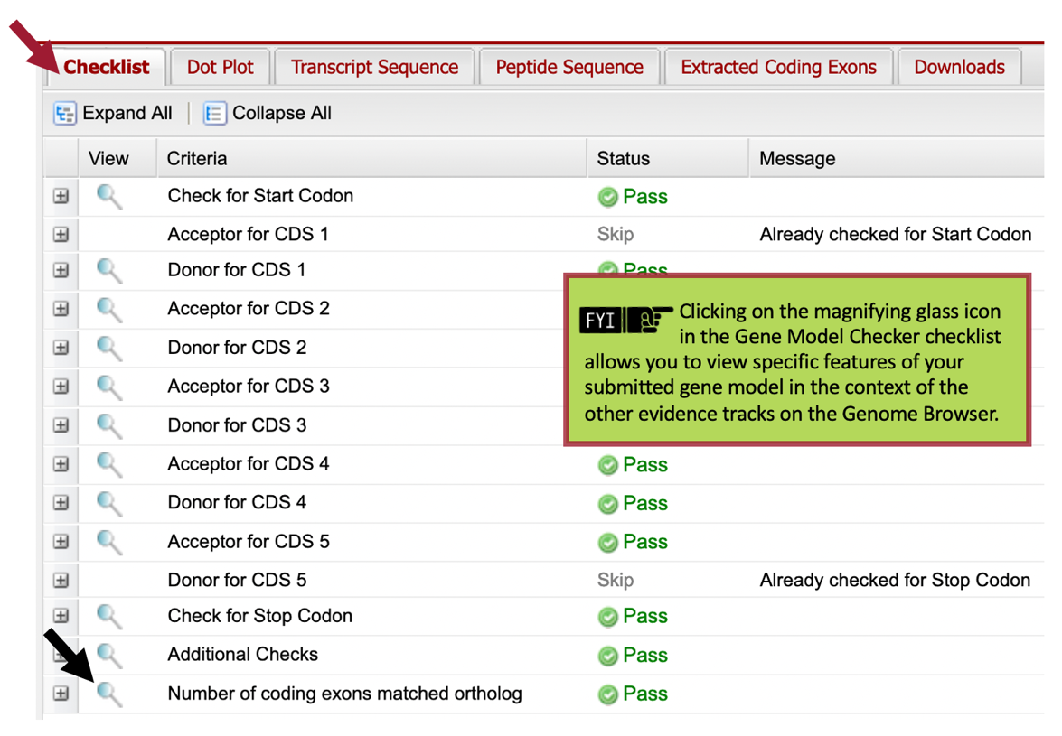
Once the analysis is complete, the right panel of the Gene Model Checker contains the results. The “Checklist” tab enumerates the list of criteria that have been checked by the Gene Model Checker (Figure 75). For example, the Gene Model Checker verifies that our proposed gene model begins with a start codon and ends with a stop codon. It also verifies that the splice junctions contain the canonical (“standard”) splice donor (GT) and acceptor (AG) sites. Some of the items on the checklist have been skipped because they do not apply to a complete gene (e.g., CDS-1 doesn’t have a splice acceptor site and CDS-5 doesn’t have a splice donor site).
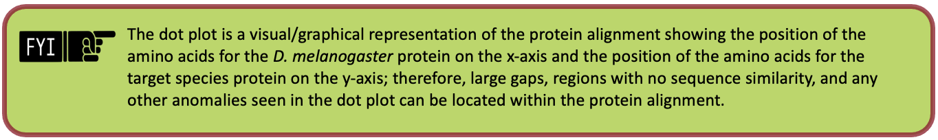
In addition to verifying the basic gene structure, the Gene Model Checker also compares the proposed gene model against the putative D. melanogaster ortholog using a protein alignment and a dot plot (Figure 77).
The alternating color boxes in the dot plot correspond to the different CDS’s in the two sequences. Dots in the dot plot correspond to regions of similarity between the D. melanogaster protein and the submitted D. yakuba gene model. If the submitted sequence is identical to the D. melanogaster ortholog, then the dot plot will show a straight diagonal line with a slope of 1. Changes in the size of the submitted model compared to the D. melanogaster ortholog will alter the slope of this line.
In this case, the dot plot shows that the five CDS’s of Rheb-PA in D. melanogaster and D. yakuba have similar lengths (compare the length shown on the x-axis to the length shown on the y-axis for each CDS). However, within a small region of CDS-4, the dot plot did not detect sequence similarity between the submitted model for D. yakuba and the D. melanogaster ortholog (Figure 76).
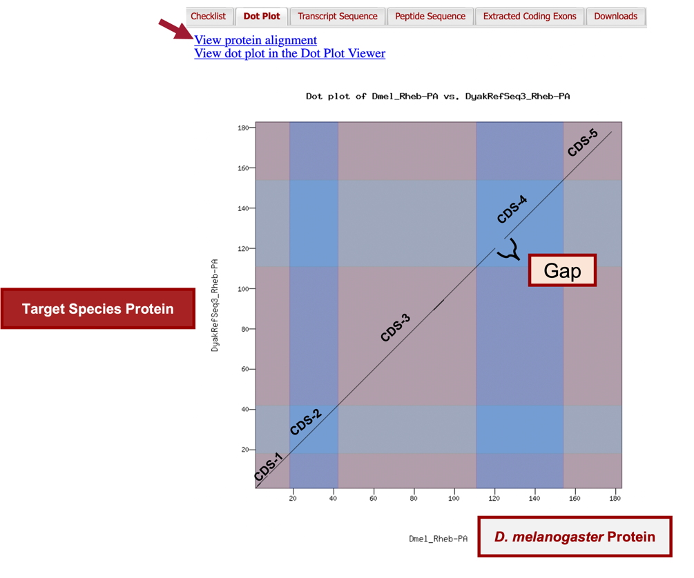
To further investigate the dot plot, we will examine the protein alignment between the two sequences.
-
Click on the “View protein alignment” link above the dot plot (Figure 76, arrow).
The protein alignment shows the comparison of the D. melanogaster protein against the conceptual translation for the submitted D. yakuba gene model. Like the dot plot, alternating colors correspond to the different CDS’s (Figure 78).
The protein alignment between the D. melanogaster ortholog and the D. yakuba gene model shows that the five CDS’s are 97.3% identical. The symbols in the match line denote the level of similarity (“*” indicates conserved amino acids, “:” denotes amino acids with highly similar chemical properties). Hence, the tiny gap in the dot plot within CDS-1 can be attributed to similar, but not identical, amino acids near its center.

The protein alignment between the D. melanogaster Rheb-PA and the submitted gene model in D. yakuba shows that that the gap within CDS-4 in the dot plot can be attributed to differences in three amino acid residues.
We can view the submitted gene model within the context of the other evidence tracks in the Genome Browser.
Now we see our entire submitted gene model for Rheb-PA in D. yakuba (Figure 80).

Part 7.2: Download files required for project submission
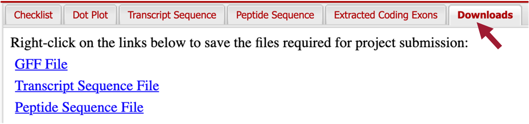
In addition to the Pathways Project: Annotation Form, you must prepare three additional data files to submit a project to the GEP — a General Feature Format File (GFF), a Transcript Sequence File (fasta), and a Peptide Sequence File (pep). The Gene Model Checker automatically creates these three files for a specific isoform (e.g., Rheb-PA) when you verify a gene model.
-
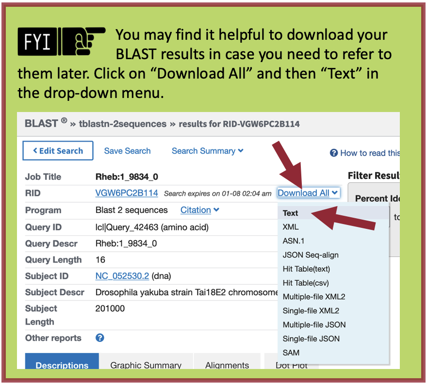
You can download these files by clicking on the “Downloads” tab and then clicking on each of the links to save the files to your computer (Figure 81).
Recall that Rheb in D. yakuba has two isoforms; the files we just downloaded were for the Rheb-PA isoform. Since the coding exons (CDS’s) for both of our isoforms are identical, we don’t need to verify any additional models. However, if your project has multiple unique isoforms (i.e., don’t all have identical coding regions) then you should repeat Parts 7.1 and 7.2 for each unique isoform.
Part 7.3: Merge project files
Now we need to combine the GFF, transcript sequence, and peptide sequence files for all unique isoforms into a single file prior to project submission (we’ll submit one merged file for each file type). We do NOT need to do this for Rheb in D. yakuba; however, we are including the steps for merging two separate files, so you’ll know how to do so. Again, if your project had only one unique isoform, you’d be done at this point. The following is merely to show you how to merge your files IF your project had multiple unique isoforms.
-
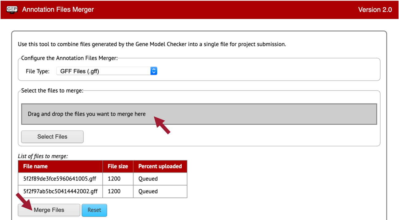
Open a new web browser tab and navigate to the Annotation Files Merger.
Let’s merge our two isoform GFF files first.
-
Change the “File Type:” to “GFF Files (.gff).”
-
Drag the two GFF files we downloaded for Rheb-PA and Rheb-PB to the “Drag and drop the files you want to merge here” section.
-
Click on the “Merge Files” button (Figure 82).
-
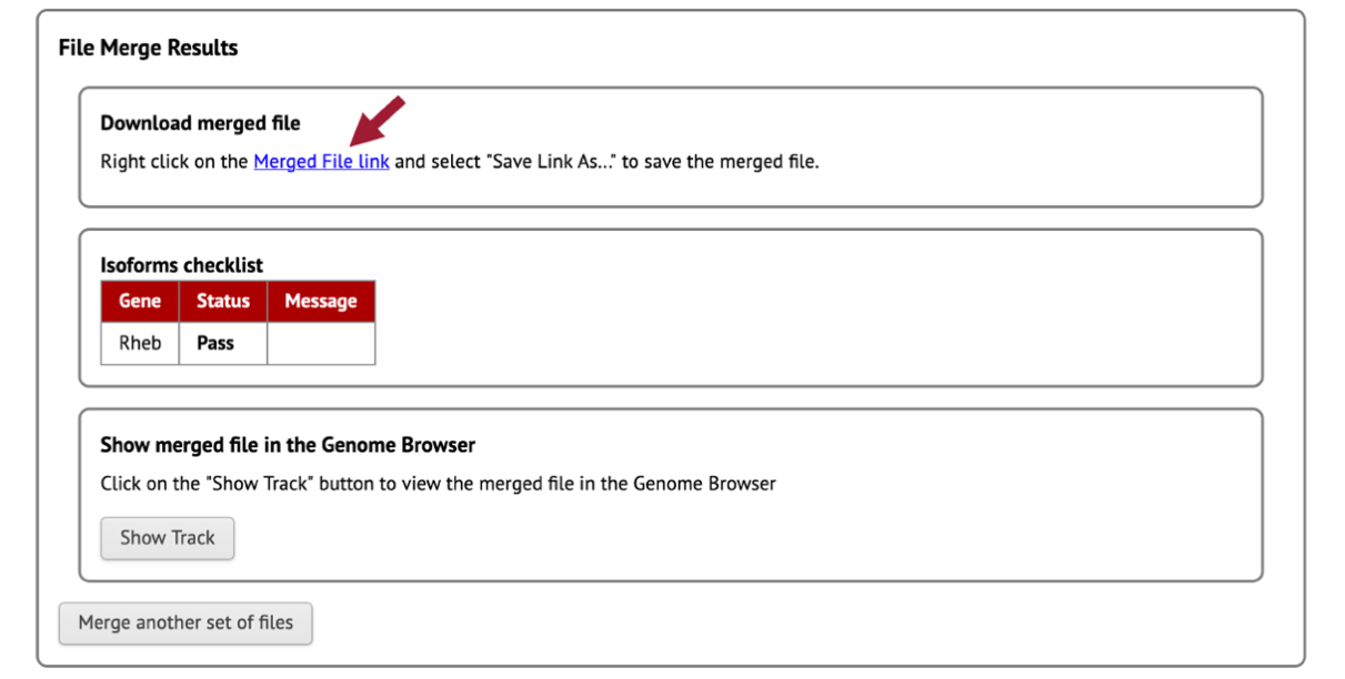
Download the merged GFF file by right-clicking (control click on macOS) on the “Merged File Link” (Figure 83).
-
Click on “Save Link As …”
-
Enter “dyak_Rheb.gff” as the file name.

If you are working on a different gene, use your assigned species (“d” followed by the first three letters of your species) + “_gene.filetype” as the format. For example, if you’re annotating Ilp8 in D. grimshawi, the merged GFF would be titled “dgrim_Ilp8.gff” -
Once you click on the “Save” button, the merged GFF file should download onto your computer.
Now we need to merge our two isoform Transcript Sequence Files (.fasta).
-
Click on the “Merge another set of files” button.
-
Change the “File Type:” to “Transcript Sequence Files (.fasta).”
-
Drag the two fasta files we downloaded for Rheb-PA and Rheb-PB to the “Drag and drop the files you want to merge here” section.
-
Repeat steps 4 – 6.
-
Enter “dyak_Rheb.fasta” as the file name.
-
Once you click on the “Save” button, the merged fasta file should download onto your computer.
Lastly, we need to merge our two isoform Peptide Sequence Files (.pep).
-
Click on the “Merge another set of files” button.
-
Change the “File Type:” to “Peptide Sequence Files (.pep).”
-
Drag the two pep files we downloaded for Rheb-PA and Rheb-PB to the “Drag and drop the files you want to merge here” section.
-
Repeat steps 4 – 6.
-
Enter “dyak_Rheb.pep” as the file name.
-
Once you click on the “Save” button, the merged pep file should download onto your computer.
Appendix A. Combining (or Batching) BLAST Searches
In Part 3.2, instead of running four individual blastp searches of the protein IDs of the nearest two neighbors upstream and downstream of the target gene, we could have combined all these searches (i.e., batched them) into a single search. Please note that this time saving method may be confusing for novice annotators.

In Part 5, instead of running five individual tblastn searches (one for each CDS), we could have entered all five CDS sequences into the “Enter Query Sequence” text box and performed all five searches at once.