Cover Sheet
Objectives
-
Identify splice donor and acceptor sites that are best supported by RNA-Seq and TopHat splice junction predictions.
-
Utilize the canonical splice donor and splice acceptor sequences to identify intron-exon boundaries.
Prerequisites
-
Define pre-mRNA as the RNA that results from the process of transcription; this initial transcript includes exons and introns
Class Instruction
-
Review pre-mRNA processing using appropriate figures from the textbook or Module 3
-
Investigation 1: Students familiarize themselves with RNA-Seq data
-
Review consensus sequences for splice donor and splice acceptor sites
-
-
Investigation 2: Students find splice donor and acceptor for intron 1
-
Review RNA splicing of intron 1 using tra-RA as the example
-
-
Investigation 3: Students find remaining splice donor and splice acceptor for intron 2
-
Discuss length of pre-mRNA vs. length of spliced mRNA
-
Identify isoforms with different TSSs or alternative splicing patterns
-
Associated Videos and Resources
Investigation 1: Examining RNA-Seq data
We will continue to focus on isoform A of transformer (referred to as tra-RA). Here we will focus on data from experiments that assess the RNA population in cells. This data can be used to help us identify exons and introns for the gene under study.
All RNAs in the cell are collectively known as the “transcriptome,” as almost all RNA is produced by transcription from a DNA template (in some cases, RNA is made from an RNA template). The transcriptome includes messenger RNAs (mRNAs), ribosomal RNAs, transfer RNAs, and other RNAs that have specialized functions in the cell.
RNA can be harvested from cells or a whole organism like Drosophila and converted to DNA, then sequenced to produce RNA-Seq (RNA Sequencing) data. First, extracted mRNA that has been fully spliced is copied back to DNA with the enzyme called reverse transcriptase. Short fragments of the copied or complementary DNA are sequenced, and then these segments are mapped back to the genome. By analyzing the mapping data, it is possible to know which and how many mRNA molecules have been transcribed.
This is a powerful technique that allows us to see when, where, and how much different genes are expressed. This kind of information can help researchers and clinicians know which genes show changes in expression levels in different types of cancers, for example. Here and in the next modules we are going to use RNA-Seq data to explore how the transformer (tra) gene is expressed in male vs. female Drosophila.
RNA-Seq data can indicate where transcription occurs, to the exact nucleotide. Remember from Module 3 that the initial mRNA transcripts are quickly processed to remove the introns. Hence in total mRNA from a cell, sequences from exons will be much more abundant than sequences from introns. We will use RNA-Seq data to help us find the exon-intron boundaries for tra-RA, the isoform of the tra gene that is expressed in female fruit flies.
-
Open a new web browser window and go to the GEP UCSC Genome Brower Mirror site at gander.wustl.edu.
-
Select the “Genome Browser” link from the left side panel. (Detailed instructions for navigating to the Genome Browser Gateway page are given in Module 1.)
Reminder: use the dropdown menus on the Genome Browser to select the following:
-
Select “D. melanogaster” under the “UCSC SPECIES TREE AND CONNECTED ASSEMBLY HUBS” field.
-
Select “July 2014 (Gene)” in the “D. melanogaster Assembly” field.
-
Enter “contig1” in the “Position/Search Term” field.
-
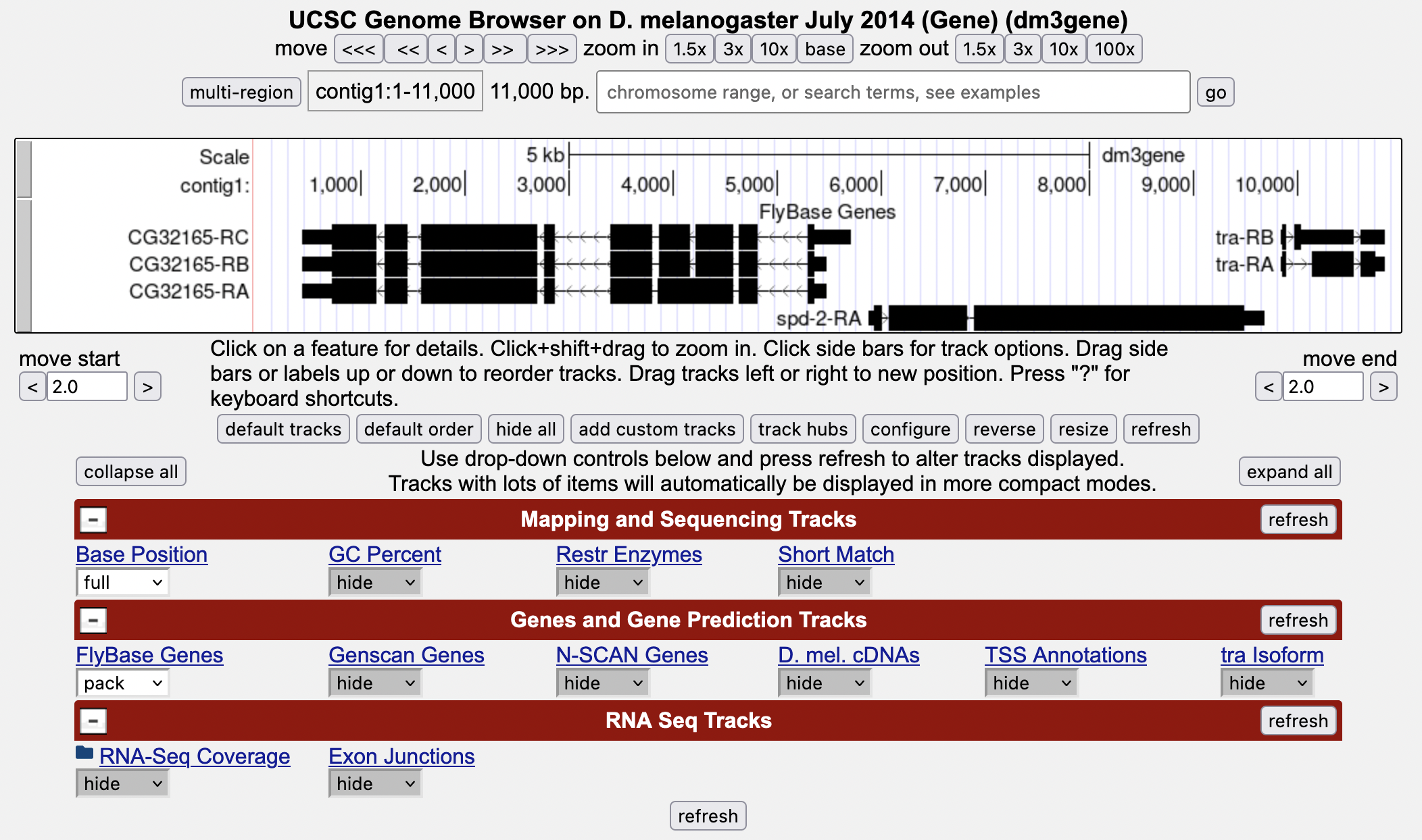
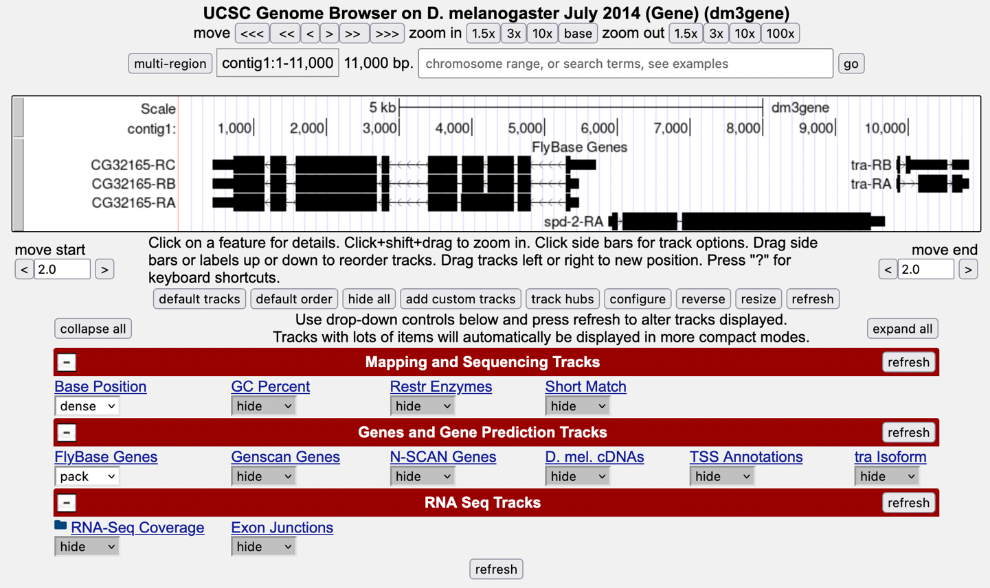
Then click “GO” and the screen below will appear (Figure 1). As you will remember, this section of DNA is 11,000 base pairs long and is part of the left arm of chromosome 3, which is about 28,100,000 bp long. If your Browser window is showing other evidence tracks, reset by clicking on “default tracks.”
-
Let’s start by setting the evidence tracks we want to see. Click on the “hide all” button. Then open only the tracks that will provide data for this investigation. Note that you will not be able to see the DNA sequence until you “zoom in.”
-
Change the “RNA-Seq Coverage” track to “full,” then click “refresh.”
You will see blue and red histograms representing RNA-Seq data generated using mRNA samples from adult females and adult males, respectively. This allows us to infer the pattern of mRNA synthesis, and to look for similarities and differences between the sexes, both of which are apparent!
-
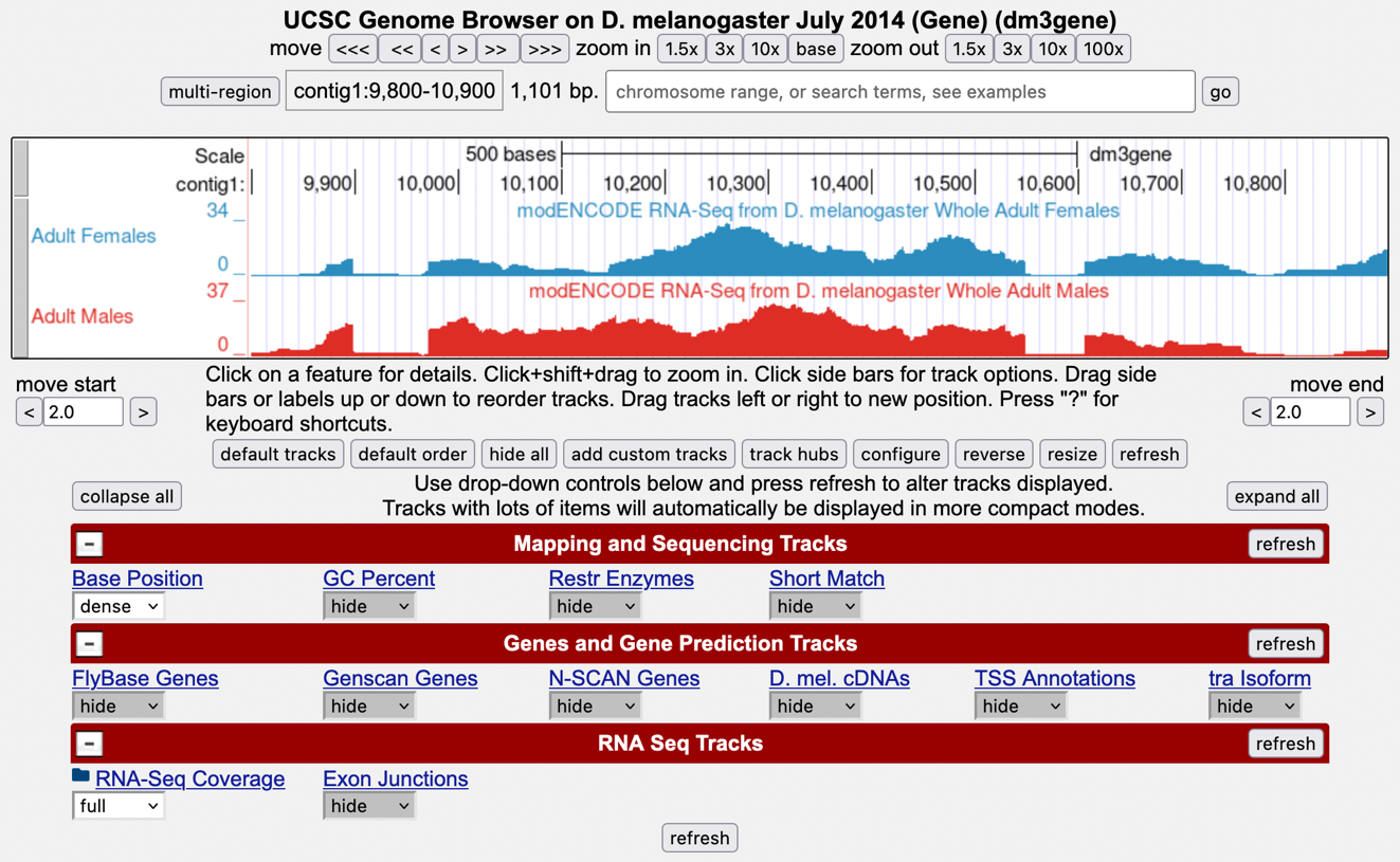
Zoom in to view only the tra gene by entering contig1:9,800-10,900 in the “chromosome range, or search terms, see examples” text box (Figure 2).
-
We are now looking at the region of chromosome 3 where the tra gene is located. Compare the blue and red histograms for the adult females and adult males RNA-Seq samples. Note that there are numbers on the y-axis that show how many RNA reads (sequences from transcripts) map to that position.
List two ways in which the histograms are similar.
List one way that the histograms differ (other than color).
To recap: The blue histogram represents the sequenced mRNA from female fruit flies and represents the form of the tra gene referred to as isoform A (tra-RA). The red histogram represents the RNA-Seq data from male fruit flies, which differs from that in females; this represents a second isoform of the tra gene called tra-RB.
Recall that our other evidence (see Module 3) indicates that tra-RA (blue, female-specific) extends from 9,851 to 10,846. How many gaps do you see in the histograms in this interval?
Each gap corresponds to an intron — there is very little RNA-Seq signal for that part of the gene because the intronic RNA was spliced out before the mRNA was collected and sequenced.
|
|
Notice that in the first intron, the RNA-Seq histogram for tra-RA (blue, female-specific) has a long stretch of very low bars, which are much shorter than the bars for the expressed exons, and much shorter than the corresponding region in the red histogram of RNAs from male fruit flies. This region is part of the intron in female flies, and it reflects the alternative splicing event that creates the female-specific isoform. However, because a small fraction of the RNA-Seq reads is derived from pre-mRNAs, we can still find intronic sequences in RNA-Seq data. We can use a subset of the RNA-Seq reads that span adjacent exons to verify that this region is part of the intron in the mRNAs produced by female flies (e.g., exon junction predictions derived from spliced RNA-Seq reads, discussed next in Investigation 2). |
How many exons do you see?
Remember that the exon is the “expressed” part of the gene and there will be either a sharp, or broad, peak in the RNA-Seq histogram.
Do females or males make more transformer mRNA, or do they express it at about the same level?
Now that you’ve examined the evidence yourself, let’s go back and review.
-
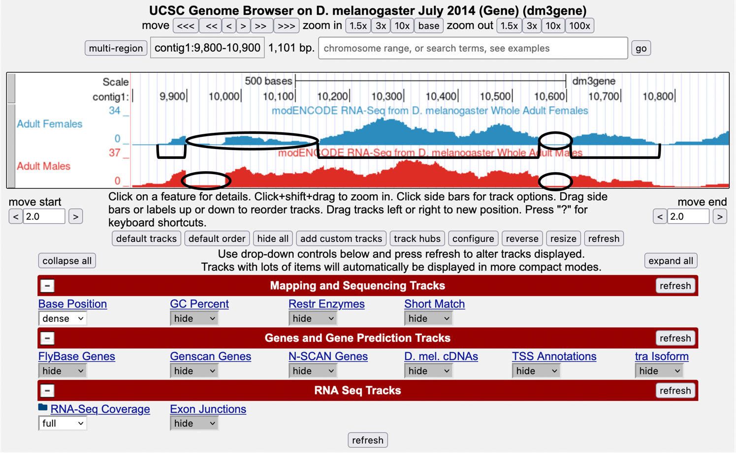
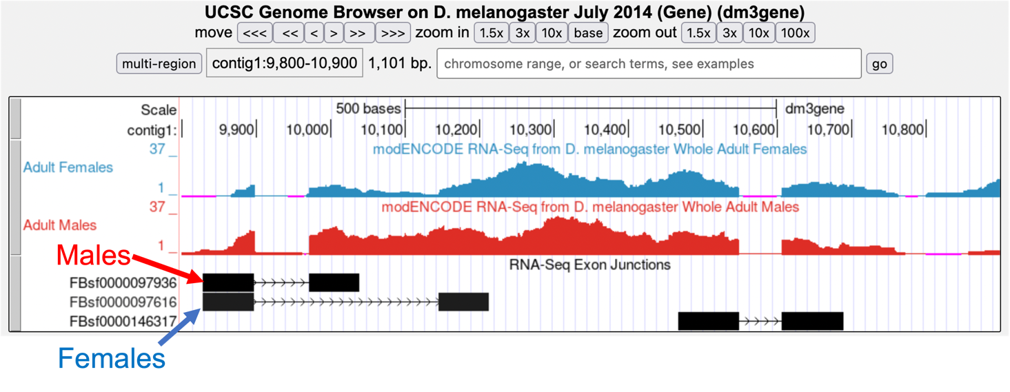
Gaps (introns) — Figure 3 is a screenshot of the Genome Browser with gaps circled. Note that there are 2 gaps in females, and 2 gaps in males. The first gap in females looks a little strange because it doesn’t have clean boundaries, suggesting a mixed population of processed transcripts.
-
Exons — Brackets have been drawn underneath the RNA-Seq data for Adult Female flies, corresponding to the three exons that are expressed.
-
Isoforms — Note that isoform A and isoform B of the tra gene are the result of alternative splicing. For some genes, isoforms may instead have different transcription start sites. Isoforms of a gene always have different mRNA sequences, but they may have the same protein sequence. To learn more about isoforms and genes, watch the Genes and Isoforms video.
Using the information you’ve gathered so far, make a diagram of the tra-RA (female-specific) isoform with 3 exons and 2 introns. Represent exons as rectangular boxes and introns as lines connecting the boxes. Number each exon and intron (start from the left with “exon 1”).
Where is the promoter in relation to the exons and introns?
|
|
On your diagram, mark the putative Transcription Start Site in your diagram with a bent arrow pointing in the direction of transcription. |
Investigation 2: Identifying splice sites
We will again focus on tra-RA to identify splice sites, that is, the exact nucleotides where splicing occurs to remove introns from the pre-mRNA.
Background
Two software programs, called TopHat and Bowtie, use the RNA-Seq data to graphically represent the exon junctions. The resulting graphic on the Genome Browser coincidentally looks something like a little bowtie (two small boxes connected by a thin line) (Figure 4). The boxes represent the sequenced mRNA (the exons), and the line represents a gap (the intron). The exon junction can be inferred when the first part of a sequenced fragment from the RNA population matches (for example) DNA positions 50-100 and the second part of the same fragment matches DNA positions 200-250; the RNA from positions 101-199 must have been taken out of the middle!
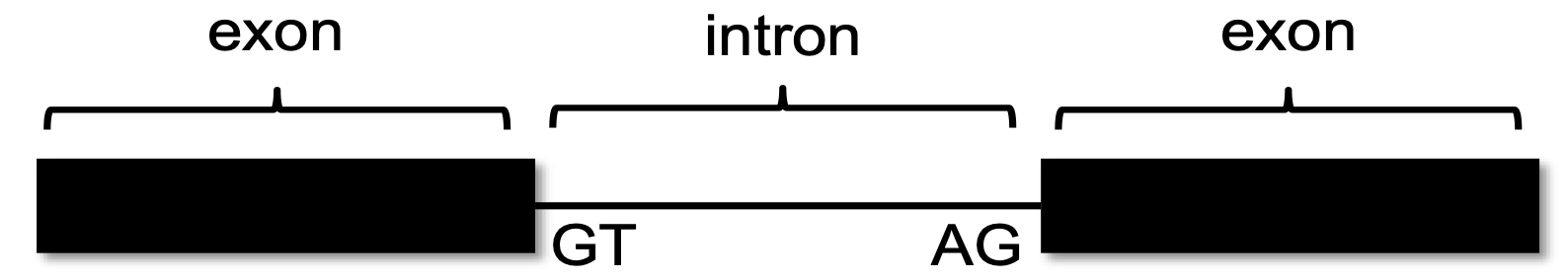
Short sequences are present at the beginning and end of each intron that allow the spliceosome—the molecular machinery that cuts out introns—to precisely remove the intron, leaving only the exon sequences in the mature mRNA. The first two nucleotides of the intron are the splice donor site and almost always the nucleotides “GT”. The last two nucleotides of the intron are the splice acceptor site and almost always the nucleotides “AG”(recall your observations in Module 3). For more information on RNA-Seq and the search for splice junctions, watch the RNA-Seq and TopHat video.
-
Using the same Genome Browser page, reset the Browser by clicking on “hide all.” Then open the tracks that will provide the information we want for Investigation 2.
|
|
If you stopped after Module 4: Investigation 1, then you may want to return to page 2 for a reminder panel of how to get to the Genome Browser page. |
-
Change the “Base Position” track to “dense.”
|
|
Note that you will not be able to see the DNA sequence until you “zoom in.” |
-
Change the “RNA-Seq Coverage” track to “full,” then click “refresh.”
You will again see blue and red histograms representing the RNA-Seq data (indicating the amount of mRNA transcribed) in females and males, respectively. We will focus on the blue histogram (Adult Females) again.
-
As we did in Module 3, let’s customize the RNA-Seq track by setting the “Data view scaling” field to “use vertical viewing range setting” and the “max” field under “Vertical Viewing range” to 37. Remember that you gain access to these settings by clicking on the “RNA-Seq Coverage” link under the RNA-Seq Tracks red bar.
-
Change Exon Junctions to “full,” then click “refresh.”
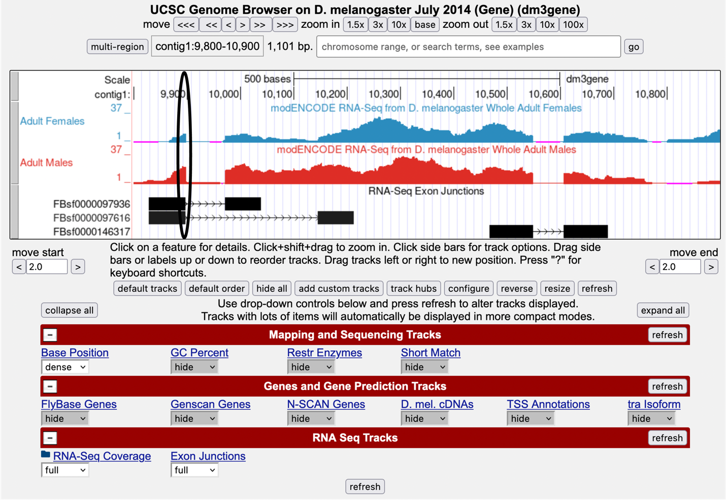
The rectangular boxes joined by a thin black line will help you identify the exon-intron boundaries. Our graphical output viewer will look like the screenshot below (Figure 5).
-
Zoom in to the area that is circled — click and drag the cursor just above the numbers, or use zoom buttons.
-
Set the screen so that you can see about 15-20 nucleotides, as shown in the example below (Figure 6).
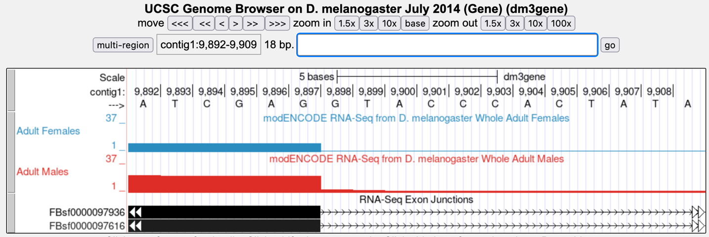
The blue histogram stops at the end of exon 1. The last three nucleotides of exon 1 are “G-A-G.”
What is the coordinate of the last nucleotide of tra-RA exon 1?
What are the first two nucleotides of tra-RA intron 1?
(This is called the 5' splice site or “splice donor site”)
-
Zoom out so that you can see all of the tra gene. Let’s use TopHat to help us find the 3' end of the intron. Examine the Exon Junctions track. The first intron-exon junction predicted by TopHat (black) seems to align with the red histogram data from males; the second junction aligns better with the blue histogram data from females (Figure 7).
-
Let’s examine the 3' end of intron 1 more closely. Change the “chromosome range, or search terms” field to contig1:10,140 and then click “go.” Zoom out 10x and then 3x (Figure 8).
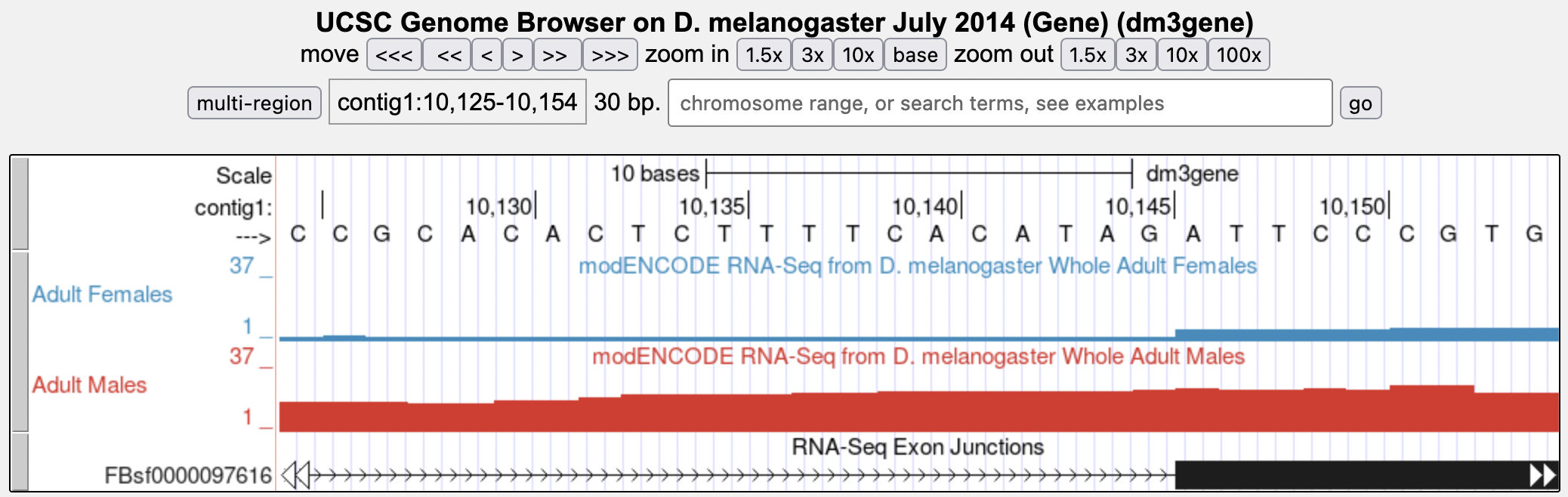
What are the last two nucleotides of tra-RA intron 1?
(This is called the 3' splice site or “splice acceptor site”)
What is the coordinate of the first nucleotide of tra-RA exon 2?
Investigation 3: Identify the 5' splice donor and 3' splice acceptor sites for intron 2
We can use the same approach to map the exon-intron boundaries of the second intron.
Review steps #2–5 in Investigation 2. Then repeat the process to answer the following questions about the 5' splice donor and 3' splice acceptor sites for the tra-RA (female-specific) intron 2.
-
Zoom into the sequence surrounding the 5' splice donor for the tra-RA (female-specific) intron 2.
What are the last three nucleotides of tra-RA exon 2?
What is the coordinate of the last nucleotide of tra-RA exon 2?
What are the first two nucleotides of tra-RA intron 2?
-
Zoom out until you can see all of intron 2. Use TopHat to find the 3' end of intron 2.
-
Click and drag so that the end of intron 2 is centered in the viewer. Then zoom in so that you can see the nucleotide sequence.
What are the last two nucleotides of tra-RA intron 2?
What is the coordinate of the first nucleotide of tra-RA exon 3?
Using the information you’ve gathered so far, make a graphical picture of the tra-RA (female-specific) isoform with 3 exons and 2 introns. Number each exon and intron at the corresponding DNA coordinates. Add the coordinates for first and last nucleotide of the exons that you have found so far. Add the sequences of the splice donor and splice acceptor sites at the appropriate locations.
Where do you think the promoter is located in relation to your gene model? What evidence do you have to support your idea, using the evidence tracks we have displayed (Base Position, RNA-Seq Coverage, Exon Junctions)?
Bonus question! Support your hypothesis by gathering additional data. Recall our explorations in Modules 2 and 3. You might want to open the tracks “D. mel. cDNAs,” and “TSS Annotations,” both in full. What type of evidence is shown by each of these tracks (refer to Module 2)? Finally, to see tra-RA as currently annotated in FlyBase, open the “tra Isoform” track on full, or to see both isoforms open the “FlyBase Genes” track in pack. Do these results support your model? Do any ambiguities remain?
Module 4 Homework: Determining splice sites for the spd-2 gene
-
Open a new web browser window and go to the GEP UCSC Genome Browser Mirror site at gander.wustl.edu.
-
Follow the instructions given in Module 1 to navigate to the contig1 project in the D. melanogaster “July 2014 (Gene)” assembly.
|
|
Reminder: use the drop-down menus on the Genome Browser to select the following:
|
Then click “GO” and the screen below will appear (Figure 9). As you will remember, this section of DNA is 11,000 base pairs long and is part of the left arm of chromosome 3, which is about 28,100,000 bp long. If your Browser window is showing other evidence tracks, reset by clicking on “default tracks.”
-
Let’s start by setting the evidence tracks we want to see. Click on the “hide all” button. Then open only the tracks that will provide data for this investigation.
-
Base Position “dense” — Note that you will not be able to see the DNA sequence until you zoom in. If the Base Position track is changed to “full”, you can see the amino acid tracks also.
-
RNA-Seq Coverage “full” — You will see blue and red histograms representing RNA-Seq data generated using RNA samples from adult females and adult males, respectively.
-
Exon Junctions “full” — Viewing the exon junctions will help you to find the splice donor and splice acceptor sites.
-
D. mel. cDNAs “full” — This track was used extensively in previous modules and is useful for confirming the sequence of the mature mRNA. Remember that a cDNA is a DNA copy of an mRNA.
-
Zoom in to view only the spd-2 gene by entering “contig1:5,750-9,800” in the “chromosome range, or search terms” text box.
We are now looking at the region of chromosome 3 where the spd-2 gene is located.
How many exons does spd-2 have?
How many introns does spd-2 have?
Homework Part 1: Identifying splice sites for intron 1
You remember from class that short sequences are present at the beginning and end of each intron that allow the spliceosome to precisely remove it, leaving only the exon sequences in the mature mRNA. The first two nucleotides of the intron are “GT”, and the last two nucleotides are “AG” (Figure 10).

-
Zoom in to the end of exon 1. Set the screen so that you can see about 15-20 nucleotides.
What is the coordinate of the last nucleotide in exon 1?
What are the first two nucleotides of intron 1?
-
Zoom out so that you can see all of intron 1 and use TopHat to help find the end of the intron. Examine the Exon Junctions track.
-
Then zoom in so that you can see the nucleotide sequence.
What are the last two nucleotides of intron 1?
What is the coordinate of the first nucleotide in exon 2?
Homework Part 2: Identifying the 5' splice donor and 3' splice acceptor sites for intron 2
Let’s use the same approach to map the exon-intron boundaries for intron 2.
-
Review the steps you used in Part 1, then repeat the process to answer the following questions about the 5' splice donor and 3' splice acceptor sites for intron 2.
-
Zoom in to the sequence surrounding the 5' splice donor for intron 2.
What is the coordinate of the last nucleotide in exon 2?
What are the first two nucleotides of intron 2?
-
Zoom out as needed so that you can see all of intron 2. Use TopHat to find the end of intron 2.
-
Click and drag so that the end of intron 2 is centered in the viewer. Then zoom in so that you can see the nucleotide sequence.
What are the last two nucleotides of intron 2?
What is the coordinate of the first nucleotide in exon 3?
Using the information you’ve gathered so far, make a graphical picture of the spd-2 gene with 3 exons and 2 introns. Number each exon and intron. Add the coordinates for first and last nucleotide of the exons that you have found so far. Add the sequences of the splice donor and splice acceptor sites at the appropriate locations. Finally, add a bent arrow to indicate the transcription start site and directionality.